Magnetostatics
Magnetostatics describes the relationship between electrical currents and magnetic fields. Any moving electrical charge generates a magnetic field. The magnetic field generated by a point charge $q$ traveling at a constant velocity $\vec{v}$ is,
$$\vec{B}(\vec{r})=\frac{\mu_0}{4\pi}\frac{q \vec{v} \times (\vec{r}-\vec{r}_{charge})}{|\vec{r}-\vec{r}_{charge}|^3}\hspace{1cm}\text{[T]}.$$Here $\mu_0= 4\pi \times 10^{-7}$ T m/A is the permeability constant, $\vec{r}_{charge}$ is the position of the charge and $\vec{r}$ is the position where the magnetic field is calculated. The motion of many charges moving together can be described by a current. The magnetic field generated by constant electrical currents can be calculated using the Biot-Savart law,
\begin{equation} \vec{B}(\vec{r})=\frac{\mu_0}{4\pi}\frac{I d\vec{r}_{wire} \times (\vec{r}-\vec{r}_{wire})}{|\vec{r}-\vec{r}_{wire}|^3}\hspace{1cm}\text{[T]}. \end{equation}This this the magnetic field generated by a short wire segment. The length of the wire segment is $|d\vec{r}_{wire}|$ and the direction of $d\vec{r}_{wire}$ is the direction that the current $I$ is flowing. Isolated current segments do not exist in nature. The current always has to be flowing somewhere so typically to calculate the total magnetic field, it is necessary to sum over many current segments that are connected together.
\begin{equation} \vec{B}(\vec{r})=\frac{\mu_0}{4\pi}\int\frac{I d\vec{r}_{wire} \times (\vec{r}-\vec{r}_{wire})}{|\vec{r}-\vec{r}_{wire}|^3}\hspace{1cm}\text{[T]}. \end{equation}In general, this integral must be done numerically but there are two special cases where the integral can be performed: an infinitely long straight wire and a solenoid.
Once the magnetic field is known, it can be used to calculate the force on a current carrying wire. This force can be calculated by summing the Lorentz force law $\vec{F}=q\vec{v}\times\vec{B}$ for every particle with charge $q$ and velocity $\vec{v}$ that make up the current. This force is exploited in electric motors.
If the magnetic field is known, the current density $\vec{J}$ can be determined by Ampère's law. There are two forms of Ampère's law. The differential form allows us to calculate the current density,
$$\nabla\times\vec{B}=\mu_0 \vec{J}.$$Here the curl $\nabla\times\vec{B}$ is defined as,
$$\nabla\times\vec{B}=\left(\frac{\partial B_z}{\partial y}-\frac{\partial B_y}{\partial z}\right)\hat{x}+ \left(\frac{\partial B_x}{\partial z}-\frac{\partial B_z}{\partial x}\right)\hat{y}+ \left(\frac{\partial B_y}{\partial x}-\frac{\partial B_x}{\partial y}\right)\hat{z}.$$Ampère's law can be rewritten in the integral form using Stokes's theorem. The integral form relates the line integral of the magnetic field going once around a closed curve $C$ to the current $I_{enc}$ passing through the curve,
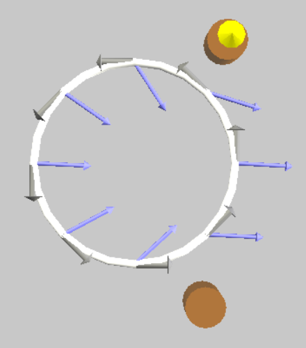
$$\oint\limits_{C}\vec{B}\cdot d\vec{l}=\mu_0 I_{enc}.$$Ampère's law can be illustrated with the following simulation.