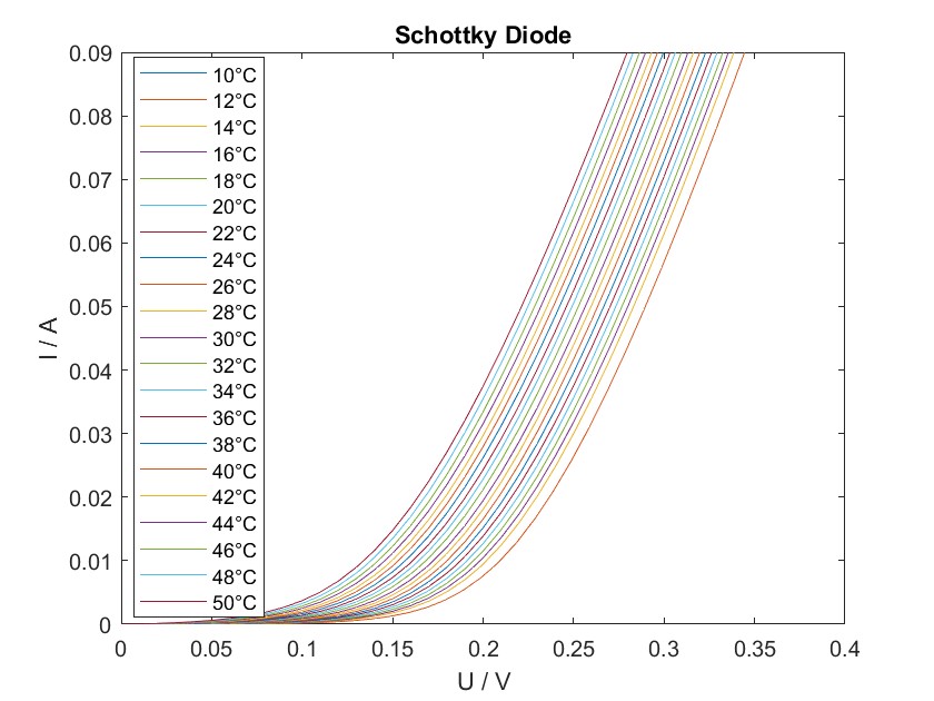
In the following experiment, the temperature dependence of the current-voltage (IV) characteristics of a Schottky diode was examined. The diode was placed in a climate chamber (Vötsch VT4002) and exposed to temperatures ranging from 10°C to 50°C. A sourcemeter (Keithley 2612A) was used to measure the IV characteristics. The ambient temperature, approximating the device temperature, and the IV data were recorded using a Python script ,which was adapted from a given template to control the instruments.
Schottky diodes are a type of semiconductor diode, but unlike pn-diodes, they do not have p-n junctions but metal-semiconductor junctions, creating a barrier known as the Schottky barrier. This barrier is a result of the difference in work function between the metal and the semiconductor. It is frequently stated that they have a lower forward voltage drop, faster switching speed and higher efficiency and reverse leakage current. However, the current-voltage characteristic of a Schottky diode has the same form as that for a pn-diode.
$$ I = I_S\left(\exp(\frac{eV}{\eta k_B T}) - 1\right)\hspace{0.5cm}\text{[A]} \tag{1}$$Here $I$ is the current, $I_S$ is the saturation current, $e$ is the charge of an electron, $V$ is the voltage, $k_B$ is Boltzmann's constant, $T$ is the absolute temperature and $\eta$ is the nonideality factor. Typically $\eta = 1$ for a Schottky diode due to the absence of recombination in the depletion region. For large voltage the last term can be neglected.
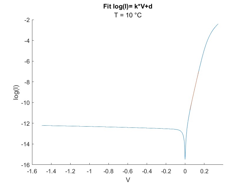
If we know take the logarithm on both sides of the equation, we get the following term:
$$ log(I) = log(I_S)+\left(\frac{e}{\eta k_B T}\right)*V\hspace{0.5cm} \tag{2} $$This now has the form of a linear function and can be written as:
$$ y=k*V + d \hspace{0.5cm}\text{with}$$ $$ k = \frac{e}{\eta k_B T} \hspace{0.5cm}\text{and} \hspace{0.5cm} d=log(I_S) \tag{3}$$ For this experiment we also want to take a closer look at the time dependency of the saturation current and the Schottky barrier. For a Schottky diode in general, the saturation current can be written as: $$I_S = \frac{Aem^*k_B^2}{2\pi^2\hbar^3}T^2\exp\left(-\frac{\phi_b}{k_BT}\right)\hspace{0.5cm}\text{[A]}$$Here $A$ is the area of the Schottky diode perpendicular to the current flow, $m^*$ is the averaged effective mass of the charge carriers, $T$ is the temperature and $\phi_b$ is the energy difference between the Fermi energy of the metal and the conduction band of the semiconductor at the interface called the Schottky barrier height. With some algebraic transformations we also get a form of an linear equation ($log (\frac{I}{T^4} ) =d + k V$). The logarithmic term is further merged to the constant $C_1$.
$$\frac{I}{T^2} = log\left(\frac{Aem^*k_B^2}{2\pi^2\hbar^3}\right)-\frac{\phi_b}{k_BT}+\frac{e}{k_BT}V \tag{4}$$ $$ \hspace{0.5cm}\text{with} \hspace{0.5cm} d=C_1-\frac{1}{k_BT}\phi_b \tag{5}$$For the experiment, the Schottky diode is placed in the heating chamber and its temperature is increased from 10 degrees Celsius to 50 degrees Celsius in steps of 2. To determine the temperature dependence of the current-voltage characteristic of a Schottky diode, the two characteristic values are recorded for the respective temperature.
In order to determine $\eta$ and $I_s$ we are going to fit the measured date with a polynom 1st order (linear fit). The two variables can be determined by transforming the fit parameters. The used range and the corresponding range selection will be further explained in Diode Analysis Discussion.
The following table displays all calculated values including uncertainties received from the fit.
| T / °C | η | Δη | I_s / A | ΔI_s / A |
|---|---|---|---|---|
| 10 | 1.002 | 0.00733 | 2.99e-06 | 7.84e-08 |
| 12 | 0.995 | 0.00728 | 2.99e-06 | 7.84e-08 |
| 14 | 0.999 | 0.00597 | 4.42e-06 | 8.50e-08 |
| 16 | 0.996 | 0.00529 | 5.24e-06 | 8.58e-08 |
| 18 | 0.990 | 0.00497 | 6.22e-06 | 9.01e-08 |
| 20 | 0.986 | 0.00432 | 7.39e-06 | 8.89e-08 |
| 22 | 0.976 | 0.00407 | 8.57e-06 | 9.18e-08 |
| 24 | 0.969 | 0.00406 | 1.00e-05 | 1.03e-07 |
| 26 | 0.961 | 0.00423 | 1.18e-05 | 1.20e-07 |
| 28 | 1.059 | 0.0189 | 2.04e-05 | 1.42e-06 |
| 30 | 1.048 | 0.0177 | 2.32e-05 | 1.47e-06 |
| 32 | 1.109 | 0.0164 | 3.36e-05 | 1.89e-06 |
| 34 | 1.111 | 0.0154 | 3.98e-05 | 2.03e-06 |
| 36 | 1.114 | 0.0145 | 4.68e-05 | 2.18e-06 |
| 38 | 1.118 | 0.0115 | 5.51e-05 | 2.46e-06 |
| 40 | 1.117 | 0.0108 | 6.41e-05 | 2.59e-06 |
| 42 | 1.115 | 0.0102 | 7.41e-05 | 2.74e-06 |
| 44 | 1.112 | 0.00957 | 8.55e-05 | 2.89e-06 |
| 46 | 1.109 | 0.00894 | 9.80e-05 | 2.98e-06 |
| 48 | 1.103 | 0.00854 | 1.13e-04 | 3.19e-06 |
| 50 | 1.097 | 0.00827 | 1.28e-04 | 3.40e-06 |
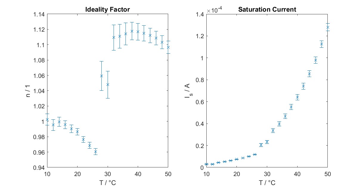
Furthermore, a graphical representation of both parameters plotted against temperature is provided.
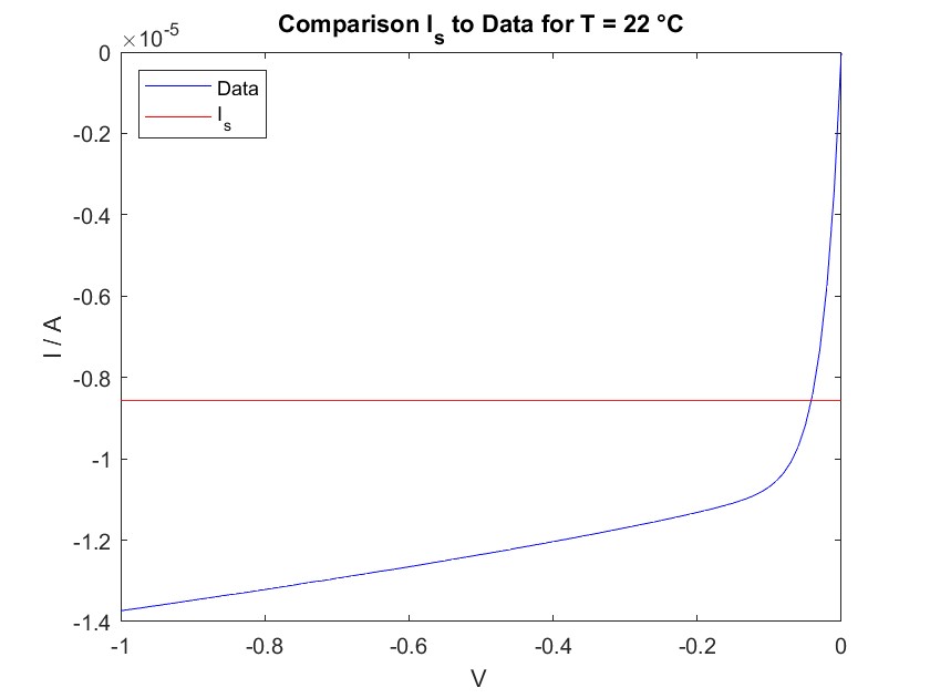
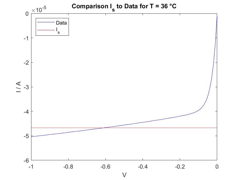
In addition, the saturation current determined from the fit is compared with the actual measured data. This is shown for two different temperatures
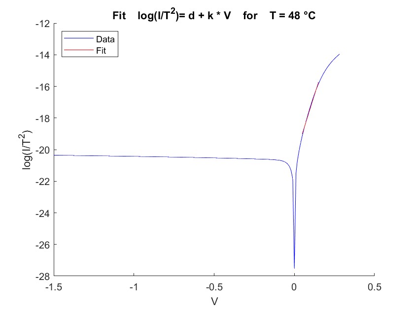
To find the Schottky barrier $\phi_b$, we divide the measured current by $T^2$ and fit it linearly, as described in formula 4. In this case, we only need the intercept for the calculation. We repeat this process for all temperatures, giving us an intercept vector that depends on temperature. Since this vector follows a linear pattern, we plot the slope against $\frac{1}{k_B T}$ and perform another linear fit. As formula 5 shows, the resulting slope represents the Schottky barrier $\phi_b$, taking its sign into account. The two fits are shown below.
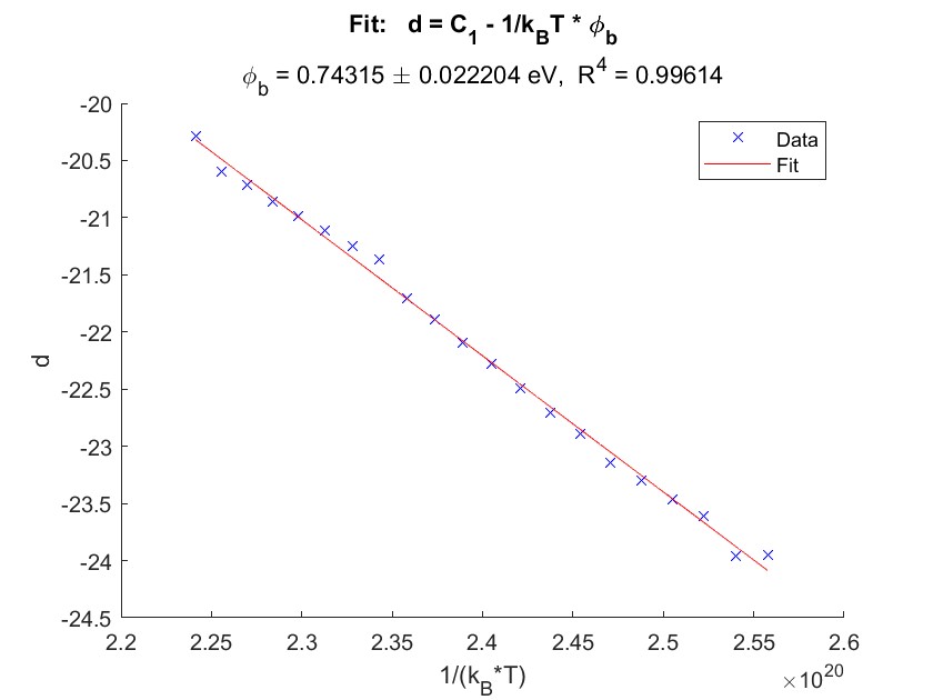
The final result for the Schottky barrier therefore is: $ \phi_b = 0.743 \pm 0.022 \mbox{ eV}$
The raw data and the generated matlab-script for plotting and fitting can be found in the linked files.
10 °C 12 °C 14 °C 16 °C 18 °C 20 °C 22 °C 24 °C 26 °C 28 °C 30 °C 32 °C 34 °C 36 °C 38 °C 40 °C 42 °C 44 °C 46 °C 48 °C 50 °C