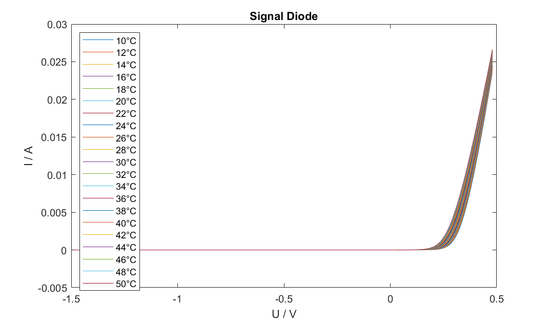
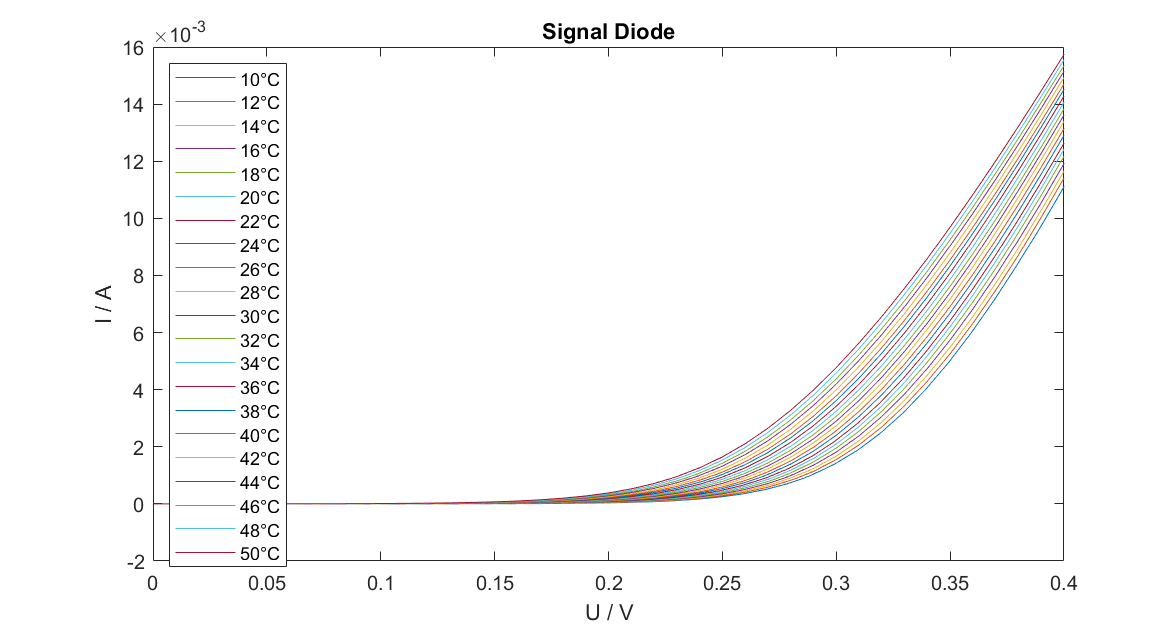
Fig.1 Plot of the measured data for every temperature.
In the following experiment, the temperature dependence of the current-voltage (IV) characteristics of a signal diode gets examined. The diode gets placed in a climate chamber (Vötsch VT4002) and exposed to temperatures ranging from 10°C to 50°C. A sourcemeter (Keithley 2612A) is used to measure the IV characteristics. The ambient temperature, approximating the device temperature, and the IV data gets recorded by using a Python script ,which is adapted from a given template to control the instruments. Further, the temperature dependent change of the behavior of the saturation current and the ideality factor gets analysed. The determined ideality factor is then used to calculate the Energy band gap of this diode.
The theory behind this analysis as well as the applied tools are explained in detail in Diode Analysis Discussion.
We use the following diode equation with the current $I$, the saturation current $I_s$, the charge of an electron $e$, voltage $V$, Boltzmann's constant $k_B$, ideality factor $\eta$ and the absolute temperature $T$.
$$ I=I_s(\exp{ (\frac{eV}{\eta k_BT} ) - 1} ) \tag{1}$$At first we will discuss, how to get the ideality factor and the saturation current from the measured data. Since we work with relatively large voltages, we can approximate formula (1) as follows.
$$I=I_s\exp{ (\frac{eV}{\eta k_BT} } ) \tag{2}$$By taking the logarithm of this equation we can achieve a linear form.
$$log(I)={log(I}_s) + \frac{eV}{\eta k_BT} \tag{3}$$We can then use formula (3) for a linear fit as $log(I)$ over $V$ for the determination of $I_s$ and $\eta$ as follows.
$$log(I)= d + k V \tag{4}$$ $$I_s=exp (d ) \tag{5}$$ $$\eta = \frac{q}{k_B T k} \tag{6}$$Since the energy band gap is only slowly changing in temperature, we assume it to be constant for this analysis. In order to determine the energy band gap Eg we have to at first include the temperature dependency. Therefore we use the following expression for $𝐼_s$
$$ I_s = A e n_i^2 (\frac{D_p}{L_p N_d}+\frac{D_n}{L_n N_a}) \tag{7} $$ $$n_i=\sqrt{N_c (\frac{T}{300} )^{3/2}N_v (\frac{T}{300} )^{3/2}}exp (\frac{-E_g}{2k_BT} ) \tag{8}$$ $$D_n=\frac{\mu_nk_BT}{e} \tag{9}$$By inserting formulas (7), (8) and (9) into the diode equation in (1) we get the following expression with the various constants all being summed up in the constant $C$
$$I=C T^4 \exp{ (\frac{eV}{k_B T} ) }exp (\frac{-E_g}{2k_BT} ) \tag{10}$$We divide this equation by $T^4$ and take the logarithm of it in order to achieve the following expression.
$$log (\frac{I}{T^4} )=log(C) + \frac{eV}{\eta k_BT} - \frac{E_g}{2k_BT} \tag{11}$$We can transform formula (11) and use it for a linear fit of $log (\frac{I}{T^4} )$ over $V$ as shown in formula (12).
$$ log (\frac{I}{T^4} ) =d + k V \tag{12}$$In order to determine the band gap, we fit the data for every temperature with formula (12). We then take the resulting intercepts $d$ and fit them again with the fit function in formula (14) as $d$ over $\frac{1}{T k_B}$.
$$d=log(a)-\frac{E_g}{2k_BT} \tag{13}$$ $$d = y_0 + m\frac{1}{T k_B} \tag{14}$$Then we can take the slope $m$ from this second fit and calculate Energy band gap from it as follows.
$$ \frac{E_g}{2} = -m \tag{15}$$For the experiment, the diode is placed in the heating chamber and its temperature is increased from 10 degrees Celsius to 50 degrees Celsius in steps of 2. We conduct a voltage sweep and measure the current and the voltage for every temperature. Figure 1 shows the measured IV-curves for every temperature.
Fig.1 Plot of the measured data for every temperature.
As shown in the plot, the IV-curves increase with temperature due to $T^4$ dominating over the exponential decay. As we would expect, the curve measured at the highest temperature is at top.
As already mentioned, we will determine $\eta$ and $I_s$ using a linear fit as in equation (4). The range used for the fit is selected via the Diode Analysis Tool, mentioned at the beginning. As figure 2 shows, the selected range is nearly perfectly linear for high temperatures as well as low temperatures.
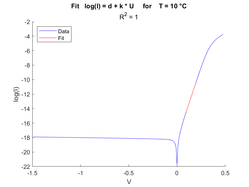
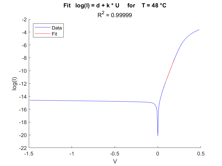
Fig.2 Fitting the IV-Curve for every temperature.
Figure 3 shows the results for $\eta$ and $I_s$ for each temperatures with the corresponding uncertainties, which result from the fit, shown as errorbars.
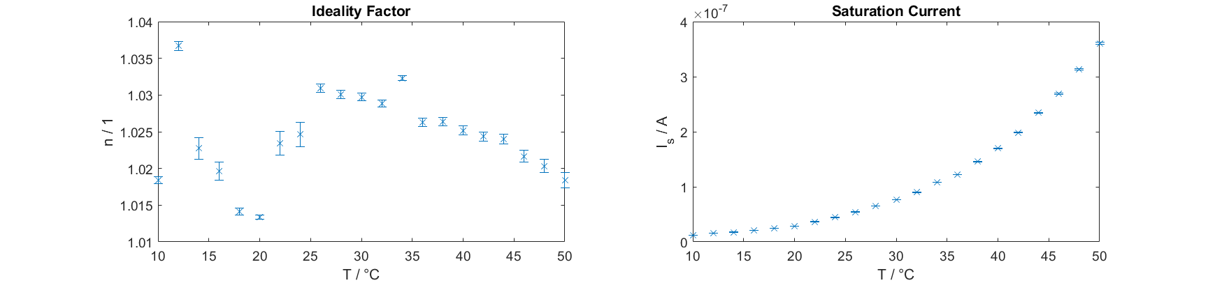
Fig.3 Results for $\eta$ and $I_s$ including uncertainties shown as errorbars
The ideality factor should be between 1 and 2 for a common signal diode. In most of the measurements we receive a value of about 1, which can be therefore seen as acceptable. Further, we also want to compare the result for $I_s$ to the measured data. Figure 4 shows the measured IV-curve at T=12° and T=48° with the corresponding $I_s$ plotted as a constant line. As it can be seen, the results fits the data quite well.
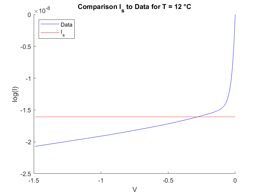
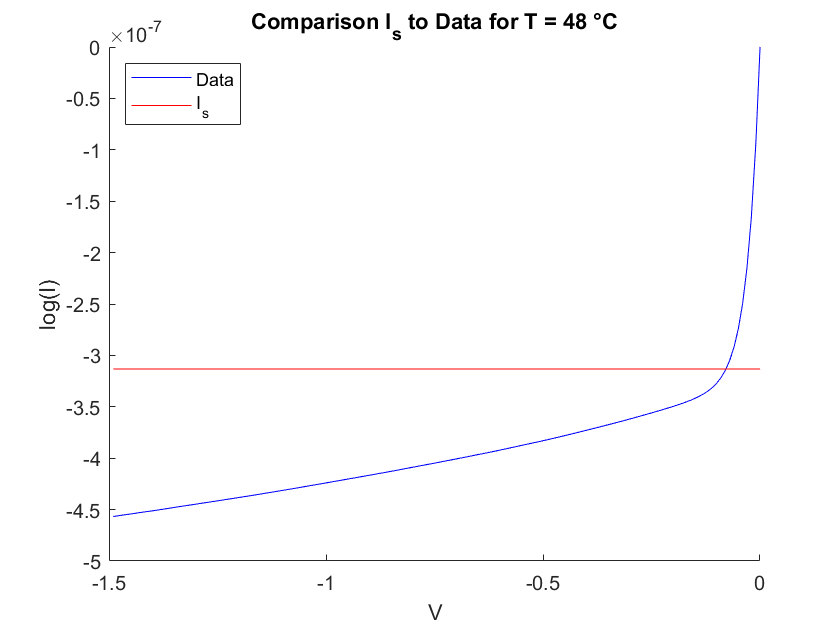
Fig.4 Comparing $I_s$ obtained by the fit to the measured data.
The following table displays all fit parameters and their corresponding uncertainties received from the fit and also $\eta$ and $I_s$ calculated from the fitparameters by using formula (5) and (6).
In order to obtain a value for the energy band gap, we will fit the data as explained in formula (12). Figure 5 shows the fit compared to the measured data for T=12° and T=48°.
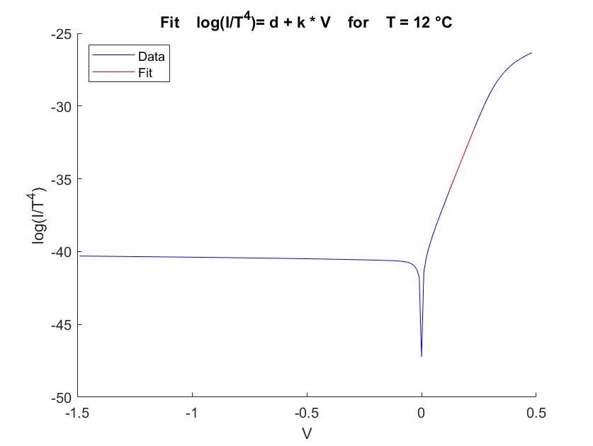
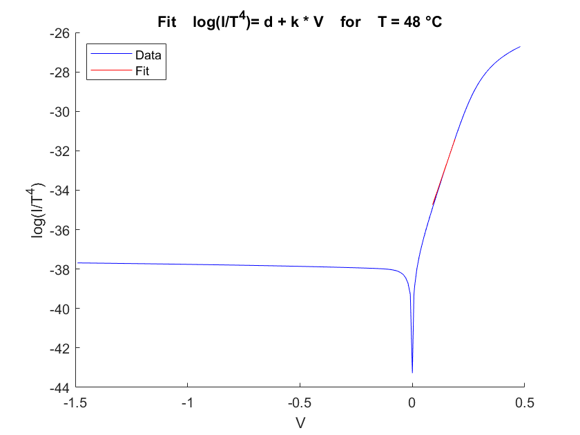
Fig.5 First Fit for obtaining $ E_g $
Then we will take the intercepts $d$ from the first fit and do a second fit with formula (14) as the fitfunction.
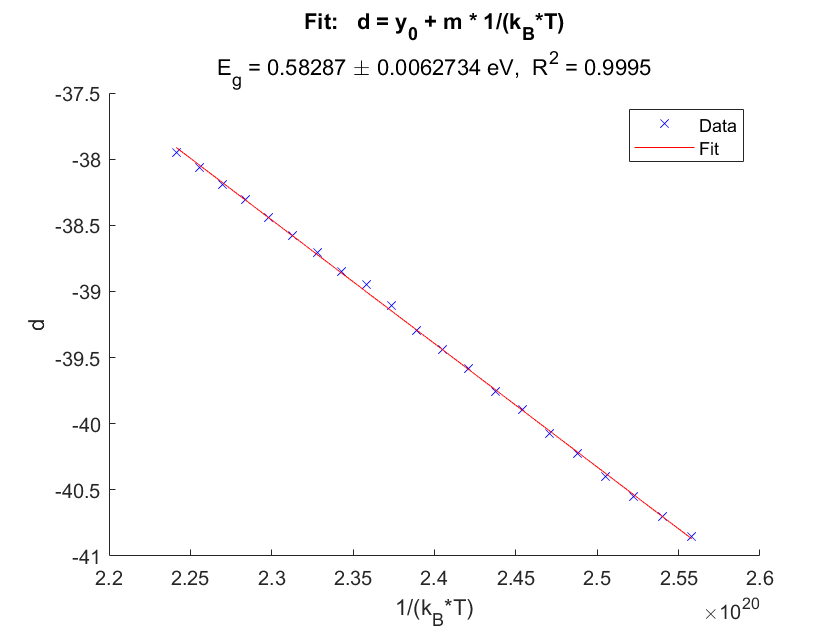
Fig.6 Second Fit for obtaining $ E_g $
With the slope of the second fit and formula (15) we obtain the final result for the energy band gap: $ E_g = 1.166 \pm 0.007 \mbox{ eV}$. This is the band gap of silicon.
10 °C 12 °C 14 °C 16 °C 18 °C 20 °C 22 °C 24 °C 26 °C 28 °C 30 °C 32 °C 34 °C 36 °C 38 °C 40 °C 42 °C 44 °C 46 °C 48 °C 50 °C