Measurements on an n-Channel MOSFET

Course: Laboratory Course Semiconductor Processing and Nanotechnology (MAS.301)
Group A3: Arthur Rönfeld, Christoph Huber & Fabian Gosdam
Period: Winter 2021
Date: 14.12.2021
Instructor: Karin Zojer

1. Introduction

The goal of this exercise was to measure and characterize a ZVN2106A n-Channel MOSFET over a range of temperatures. To become familiar with the measurement setup we first measured the saturation- and transfer characteristics of the MOSFET.

2. Measurement Setup

The Measurements were carried out using a Keithley 2600 Series Sourcemeter. We used the two channels SMU-A (Drain-Source Contact) and SMU-B (Gate-Source Contact) to power and measure the MOSFETs saturation and transfer characteristics.

    |---------------------------------|
    |                                 |
    |                                 | d
    |                            g \|-
    |            -----------o------||  N-MOS
    |            |                 ||_
  -----        -----                  | s
  | A | SMU    | B | SMU              |
  -----        -----                  |
    |            |                    |
    -------------o----------o----------
Figure 1: Measurement Setup

In order to produce different temperature environments a Vötsch VT4002 climate chamber was used.

3. Measurements

3.1 Saturation characteristics

The saturation characteristics for different Gate-Source Voltages are shown in Figure 2. The python code used to produce them is shown below.

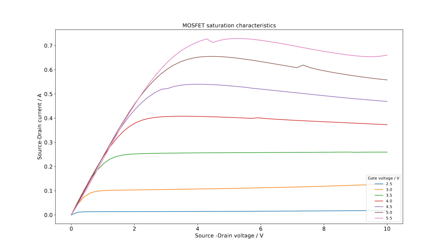
Figure 2: Output/Saturation Characteristics
[MOSFET_Ambient_saturation.npy]
Source-Drain current plottet against the Source-Drain voltage for different Gate-voltages.
from KeithleyV15 import SMU26xx
from setupElab import eLabFTW
import matplotlib.pyplot as plt
import time
import csv
import datetime
import numpy as np
""" EXAMPLE: Saturation-(Output) chracteristics of a n-channel MOSFET  

    |---------------------------------|
    |                                 |
    |                                 | d
    |                            g \|-
    |            -----------o------||  N-MOS
    |            |                 ||_
  -----        -----                  | s
  | A | SMU    | B | SMU              |
  -----        -----                  |
    |            |                    |
    -------------o----------o----------
"""

""" ******* Experiment description and plot names for eLab ******* """

test_condition = 'Ambient'
plot_name = 'MOSFET saturation characteristics'
exp_title = "n-type MOSFET characteristics"
exp_description = "Transfercharacteristic of a n-type MOSFET"

exp_date = datetime.datetime.now().strftime("%Y_%m_%d")

# Connect to eLab and create an experiment
elab = eLabFTW()
elab.set_experiment(exp_title, exp_date,  exp_description)

""" ******* Connect to the Sourcemeter ******** """

# initialize the SM and connect to it
sm = SMU26xx("TCPIP0::129.27.158.188::inst0::INSTR")

# enable the debug output (= lots of print commands)
# smu.enable_debug_output()

# get the two channels of the smu
smua = sm.get_channel(sm.CHANNEL_A)
smub = sm.get_channel(sm.CHANNEL_B)

# Create unique filenames for saving the data

time_for_name = datetime.datetime.now().strftime("%Y_%m_%d_%H%M%S")
filename_csv = 'MOSFET' + test_condition + time_for_name +'.csv'
filename_pdf = 'MOSFET' + test_condition + time_for_name +'.pdf'

# Header for csv
with open(filename_csv, 'a') as csvfile:
        writer = csv.writer(csvfile, delimiter=';',  lineterminator='\n')
        writer.writerow(["Voltage / V", "Current / A"])

""" ******* Configure the SMU Channel A (Drain-Source) ******** """

# reset to default settings
smua.reset()
# setup the operation mode and what will be shown at the display
smua.set_mode_voltage_source()
smua.display_current()

# set the measurement speed to med (so we can sweep really faster than in normal mode)
smua.set_measurement_speed_med()

# define variables we store the measurement in
data_current = []
data_voltage = []

# maximum value for source drain current
limit = 1E-1

# define the initial parameters for the channel
smua.set_voltage_range(20)
smua.set_voltage_limit(20)
smua.set_voltage(0)
smua.set_current_range(limit)
smua.set_current_limit(limit)
smua.set_current(0)

""" ******* Configure the SMU Channel B (Gate-Source) ******** """

# reset to default settings
smub.reset()
# setup the operation mode and what will be shown at the display
smub.set_mode_voltage_source()
smub.display_voltage()

# set the measurement speed to med (so we can sweep really faster than in normal mode)
smub.set_measurement_speed_med()

# define the initial parameters for the channel
smub.set_voltage_range(20)
smub.set_voltage_limit(20)
smub.set_voltage(0)
smub.set_current_range(1E-6)
smub.set_current_limit(1E-6)
smub.set_current(0)

""" ******* do the actual measurement ******** """

# define base currents we want to run the sweep on
#voltage_steps = [3,3.5,3.6,3.7,3.8,3.9,4]
voltage_steps = np.arange(2.5,6,0.5)
#voltage_steps = np.array([1,2,3.5])
#voltage_steps = np.array([3.7])

# define sweep parameters for the collector emitter voltage
voltage_start = 0
voltage_end = 10
settling_time = 0
sweep_steps = 50

V = np.linspace(voltage_start, voltage_end, sweep_steps)

# enable the outputs
smua.enable_output()
smub.enable_output()

plt.figure(figsize = (16,9))

smua.set_measurement_speed_hi_accuracy()

# do a voltage sweep for every gate current we defined
for bias_voltage in voltage_steps:
    # some output so that we know what the smu is doing
    print("Gate voltage = " + "{0:.2f}".format(bias_voltage) + " V")
    # set the gate voltage
    smub.set_voltage(bias_voltage)
    I = []

    # sweep and record the drain-source voltage
    for voltage_now in np.linspace(voltage_start, voltage_end, sweep_steps):
        smua.set_voltage(voltage_now)
        smua.set_current_range(limit)
        smua.set_current_limit(limit)
        
        I_test = np.abs(smua.measure_current())
        #if (I_test < 1e-7):
            #print(I_test)
        #print(I_test)
        if (I_test*10 > limit) and (I_test < 1e-8):
            smua.set_current_range(limit)
            smua.set_current_limit(limit)
            print(I_test)
        else:    
            smua.set_current_range(I_test*10)
            smua.set_current_limit(I_test*10)

        
        I_meas = smua.measure_current()
        if I_meas > 1e15:  # some currents were in the range of 1e38
            I.append(np.nan)
        else:
            I.append( I_meas ) 


    #[current, voltage] = smua.measure_voltage_sweep(voltage_start, voltage_end, settling_time, sweep_steps)
    data_voltage.append(V)
    data_current.append(I)

   
    plt.plot(V, I, label=str(np.round(bias_voltage, 2)))

        
# Write the data in a csv
##with open(filename_csv, 'a') as csvfile:
##       writer = csv.writer(csvfile, delimiter=';',  lineterminator='\n')
##       writer.writerow([V , I])
np.save(filename_csv, [data_voltage, data_current])

# disable the outputs
smua.disable_output()
smub.disable_output()

# properly disconnect from the SMU
sm.disconnect()

""" ******* Plot the data we obtained ******** """

# generate a nice looking legend
#legend = []
#for i in current_steps:
  #   legend.append("Ib = " + "{0:.2f}".format(i*1000) + " mA")
leg = plt.legend( loc='lower right')
leg.set_title('Gate voltage / V')

# set labels and a title
plt.xlabel('Source -Drain voltage / V', fontsize=14)
plt.ylabel('Source-Drain current / A', fontsize=14)
plt.title(plot_name, fontsize=14)
plt.tick_params(labelsize = 14)

plt.savefig(filename_pdf)
# show the plot
plt.show()

# Upload files to eLab
elab.upload_file(filename_csv)
elab.upload_file(filename_pdf)
elab.upload_script(__file__)
n_MOSFET_outputcurve.py

The output curves shown in Figure 1 should follow the output behavior as described by the gradual channel equations:

(1)ID=K(VGSVthVDS2)VDSVDS<VGSVth(2)ID=K2(VGSVth)2VDS>VGSVth(3)K=WLμnCox

Equation (1) describes the so called ohmic regime, Equation (2) the saturation regime. The constant K depends on the channel geometry as well as the oxide capacitance Cox and the mobility μn of the n-type carriers. The data follows the equations for Gate-Voltages below 4 V ideally. For higher Gate-Voltages the current declines even thought it should stay constant according to (2). This error occurs because we only plotted the array used as input for the source-meter to set the source-drain voltage.

Important Note on the Python code:
Measuring and recording both channels of the source-meter to avoid this error in the future.

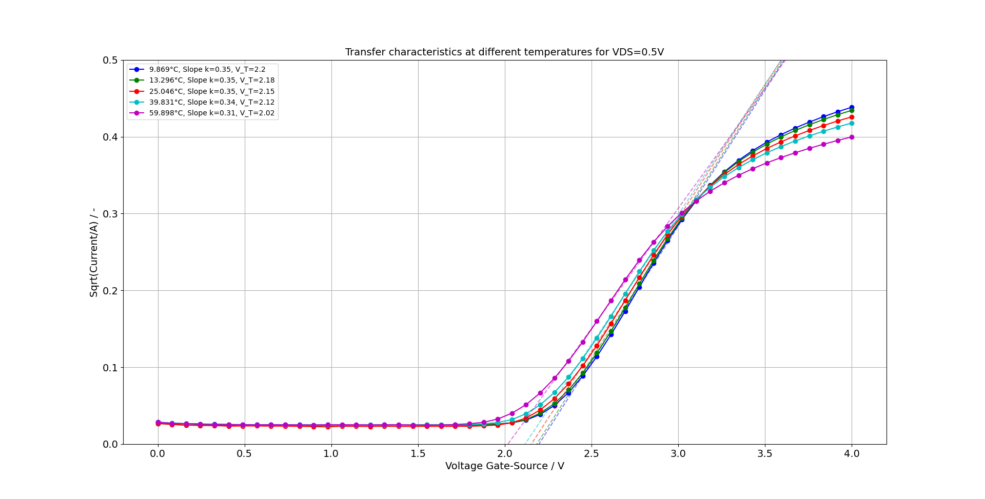
3.2 Transfer characteristics

The transfer characteristics are recorded by varying the gate-source voltage for a fixed voltage applied at across the source-drain contacts. The measured current as well as the data file, saved as numpy file format, and script used for measuring are shown in Figure 2 and below.
Figure 3: Transfer Characteristics
[MOSFET_Ambient_transfer.npy]
Source-Drain current plottet against the Gate-Source voltage for different Drain-voltages.
from KeithleyV15 import SMU26xx
from setupElab import eLabFTW
import matplotlib.pyplot as plt
import time
import csv
import datetime
import numpy as np
""" EXAMPLE: Transfer characteristics of a n-channel MOSFET  

    |---------------------------------|
    |                                 |
    |                                 | d
    |                            g \|-
    |            -----------o------||  NLDMOS
    |            |                 ||_
  -----        -----                  | s
  | A | SMU    | B | SMU              |
  -----        -----                  |
    |            |                    |
    -------------o----------o----------
"""

""" ******* Experiment description and plot names for eLab ******* """

test_condition = 'Ambient'
plot_name = 'MOSFET transfer characteristics'
exp_title = "n-type MOSFET characteristics"
exp_description = "Transfercharacteristic of a n-type MOSFET"

exp_date = datetime.datetime.now().strftime("%Y_%m_%d")

# Connect to eLab and create an experiment
elab = eLabFTW()
elab.set_experiment(exp_title, exp_date,  exp_description)

""" ******* Connect to the Sourcemeter ******** """

# initialize the SM and connect to it
sm = SMU26xx("TCPIP0::129.27.158.188::inst0::INSTR")

# enable the debug output (= lots of print commands)
# smu.enable_debug_output()

# get the two channels of the smu
smua = sm.get_channel(sm.CHANNEL_A)
smub = sm.get_channel(sm.CHANNEL_B)

# Create unique filenames for saving the data

time_for_name = datetime.datetime.now().strftime("%Y_%m_%d_%H%M%S")
filename_csv = 'MOSFET' + test_condition + time_for_name +'.csv'
filename_pdf = 'MOSFET' + test_condition + time_for_name +'.pdf'

# Header for csv
with open(filename_csv, 'a') as csvfile:
        writer = csv.writer(csvfile, delimiter=';',  lineterminator='\n')
        writer.writerow(["Voltage / V", "Current / A"])

""" ******* Configure the SMU Channel A (Gate-Source) ******** """

# reset to default settings
smua.reset()
# setup the operation mode and what will be shown at the display
smua.set_mode_voltage_source()
smua.display_current()

# set the measurement speed to med (so we can sweep really faster than in normal mode)
smua.set_measurement_speed_med()

# define variables we store the measurement in
data_current = []
data_voltage = []

# maximum value for source drain current
limit_CHA = 1E-1
limit_CHB = 200E-3

# define the initial parameters for the channel
smua.set_voltage_range(20)
smua.set_voltage_limit(20)
smua.set_voltage(0)
smua.set_current_range(limit_CHA)
smua.set_current_limit(limit_CHA)
smua.set_current(0)

""" ******* Configure the SMU Channel B (Drain-Source) ******** """

# reset to default settings
smub.reset()
# setup the operation mode and what will be shown at the display
smub.set_mode_voltage_source()
smub.display_voltage()

# set the measurement speed to med (so we can sweep really faster than in normal mode)
smub.set_measurement_speed_med()

# define the initial parameters for the channel
smub.set_voltage_range(20)
smub.set_voltage_limit(20)
smub.set_voltage(0)
smub.set_current_range(limit_CHB)
smub.set_current_limit(limit_CHB)
smub.set_current(0)

""" ******* do the actual measurement ******** """


# define sweep parameters for the drain-source voltage

#voltage_steps = [3,3.5,3.6,3.7,3.8,3.9,4]
#voltage_steps = np.arange(2.5,5.5,0.5)
V_DS = np.array([0.01,0.1,0.25,0.5])
#voltage_steps = np.array([3.7])


# define sweep parameters for the gate-source voltage
voltage_start = 0
voltage_end = 5
settling_time = 0
sweep_steps = 50

V_GS = np.linspace(voltage_start, voltage_end, sweep_steps)

# enable the outputs
smua.enable_output()
smub.enable_output()

plt.figure(figsize = (16,9))

smua.set_measurement_speed_hi_accuracy()

# do a voltage sweep for every base current we defined
for bias_voltage in V_DS:
    # some output so that we know what the smu is doing
    print("Gate voltage = " + "{0:.2f}".format(bias_voltage) + " V")
    # set the base current
    smub.set_voltage(bias_voltage)
    # sweep and record the collector emitter voltage
    # we use the build in sweep function ... which is much faster than setting every value as a separate command
    I = []


    for voltage_now in V_GS:
        smua.set_voltage(voltage_now)

##        I_test = np.abs(smua.measure_current())
##        smua.set_current_range(limit)
##        smua.set_current_limit(limit)
        #if (I_test < 1e-7):
            #print(I_test)
        #print(I_test)
##        if (I_test*10 > limit) and (I_test < 1e-8):
##            smua.set_current_range(limit)
##            smua.set_current_limit(limit)
##            print(I_test)
##        else:    
##            smua.set_current_range(I_test*10)
##            smua.set_current_limit(I_test*10)

        
        I_meas = smub.measure_current()
        if I_meas > 1e15:  # some currents were in the range of 1e38
            I.append(np.nan)
        else:
            I.append( I_meas ) 


    #[current, voltage] = smua.measure_voltage_sweep(voltage_start, voltage_end, settling_time, sweep_steps)
    data_voltage.append(V_GS)
    data_current.append(I)
    plt.plot(V_GS, I, label=str(np.round(bias_voltage, 2)))

        
# Write the data in a csv
##with open(filename_csv, 'a') as csvfile:
##       writer = csv.writer(csvfile, delimiter=';',  lineterminator='\n')
##       writer.writerow([V , I])
np.save(filename_csv, [data_voltage, data_current])

# disable the outputs
smua.disable_output()
smub.disable_output()

# properly disconnect from the SMU
sm.disconnect()

""" ******* Plot the data we obtained ******** """

# generate a nice looking legend
#legend = []
#for i in current_steps:
  #   legend.append("Ib = " + "{0:.2f}".format(i*1000) + " mA")
leg = plt.legend( loc='lower right')
leg.set_title('Source-Drain voltage / V')

# set labels and a title
plt.xlabel('Gate-Source voltage / V', fontsize=14)
plt.ylabel('Drain-Source current / A', fontsize=14)
plt.title(plot_name, fontsize=14)
plt.tick_params(labelsize = 14)

plt.savefig(filename_pdf)
# show the plot
plt.show()

# Upload files to eLab
elab.upload_file(filename_csv)
elab.upload_file(filename_pdf)
elab.upload_script(__file__)
n_MOSFET_transfer.py

3.3 Temperature dependent measurements

To measure the temperature dependence of our MOSFET we recorded the transfer characteristics once again inside the climate chamber and conducted 5 measurements.

After we measured the data we wanted to see the influence of the temperature on the threshold voltage and the mobility. According to formula (2) we see that there is a quadratic dependence of the source-drain current to the threshold voltage in the saturation regime. Therefore we plotted the y-axis as the square root of the current.
(4)ID2K=VGSVthwhereK=WLμnCox 
From (2) we know that with a higher mobility a higher current should flow. The mobility itself decreases for higher temperatures due to the increase in scattering from phonos. (Electron and hole mobility of silicon)
We extrapolated the linear range of Figure 4 to read off the threshold voltage at the intersection with the x-axis. For higher temperatures we generally got lower threshold voltages.
Figure 4: Temperature dependance of the mobility
[MOSFET_9.869°C_transfer.npy, MOSFET_13.296°C_transfer.npy, MOSFET_25.046°C_transfer.npy, MOSFET_39.831°C_transfer.npy, MOSFET_59.898°C_transfer.npy]
The dashed lines show linear fits for the range of 2.3V to 3.0V. Different slopes indicate a change in Mobility.
import numpy as np
import matplotlib.pyplot as plt

file_names = [
    'MOSFET9.869°C2021_12_14_162133.csv.npy',
    'MOSFET13.296°C2021_12_14_161029.csv.npy',
    'MOSFET25.046°C2021_12_14_155314.csv.npy',
    'MOSFET39.831°C2021_12_14_162743.csv.npy',
    'MOSFET59.898°C2021_12_14_164011.csv.npy'
]
temperatures = ['9.869°C','13.296°C','25.046°C','39.831°C','59.898°C']
path = 'Data/'
ary_sqrtcurrent = []
ary_voltage = []
poly1d_fn = []
colors = ['b','g','r','c','m']

for i,name in enumerate(file_names):
    data = np.load(path+name)
    ary_current = data[1,0,:]
    ary_voltage = data[0,0,:]
    ary_sqrtcurrent = np.sqrt(ary_current)

    # Linear rise of the voltage between 2.3 and 3.0 V
    idx = np.where((ary_voltage>2.3)*(ary_voltage<3.0))
    ary_linvoltage = ary_voltage[idx]
    ary_lincurrent = ary_sqrtcurrent[idx]

    coef = np.polyfit(ary_linvoltage,ary_lincurrent,1)
    poly1d_fn = np.poly1d(coef)
    k = np.round(coef[0],2)
    v_t = np.round((-1*poly1d_fn(0))/coef[0],2)
    # Plot the transfer curves at a certain temperature
    plt.plot(ary_voltage, ary_sqrtcurrent,'o-', label= temperatures[i] + ', Slope k=' + str(k)+ ', V_T='+str(v_t),color=colors[i])
    # Plot the linear fits at a certqain temperature
    a = np.linspace(2,4)
    plt.plot(a,poly1d_fn(a), '--',color=colors[i],alpha = 0.5)


plt.xlabel('Voltage Gate-Source / V', fontsize=14)
plt.ylabel('Sqrt(Current/A) / -', fontsize=14)
plt.title('Transfer characteristics at different temperatures for VDS=0.5V', fontsize=14)
plt.tick_params(labelsize=14)
plt.grid()
plt.ylim(0,0.5)
plt.legend()
plt.show()
mobility_fit.py