Landau theory of second order phase transitions

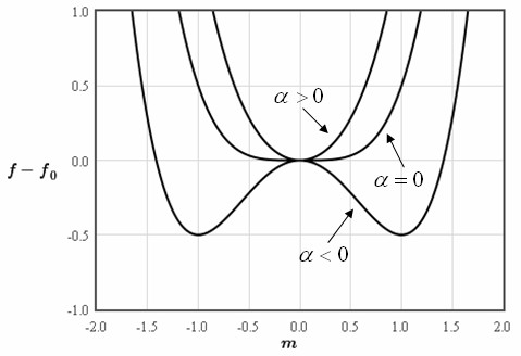
Normally, to calculate thermodynamic properties like the free energy, the entropy, or the specific heat, it is necessary to determine the microscopic states of system by solving the Schrödinger equation. For crystals, the microscopic states are labeled by k and the solutions of the Schrödinger equation are typically expressed as a dispersion relation where the energy is given for each k. The dispersion relation can be used to calculate the density of states and the density of states can be used to calculate the thermodynamic properties. This is typically a long and numerically intensive calculation.

Landau realized that near a phase transition an approximate form for the free energy can be constructed without first calculating the microscopic states. He recognized it is always possible to identify an order parameter that is zero on the high temperature side of the phase transition and nonzero on the low temperature side of the phase transition. For instance, the magnetization can be considered the order parameter at a ferromagnetic - paramagnetic phase transition. For a structural phase transistion from a cubic phase to a tetragonal phase, the order parameter can be taken to be c/a - 1 where c is the length of the long side of the tetragonal unit cell and a is the length of the short side of the tetragoal unit cell.

At a second order phase transition, the order parameter increases continuously from zero starting at the critical temperature of the phase transition. An example of this is the continuous increase of the magnetization at a ferromagnetic - paramagnetic phase transition. Since the order parameter is small near the phase transition, to a good approximation the free energy of the system can be approximated by the first few terms of a Taylor expansion of the free energy in the order parameter.

\[ \large f\left(T\right) = f_0\left(T\right)+\alpha m^2+\frac{1}{2}\beta m^4 \hspace{1cm} \alpha_0 >0, \hspace{1cm} \beta >0. \]

Here $m$ is the order parameter, $\alpha$ and $\beta$ are parameters, and $f_0\left(T\right)$ describes the temperature dependence of the high temperature phase near the phase transition. It is assumed that $\beta>0$ so that the free energy has a minimum for finite values of the order parameter. When $\alpha>0$, there is only one minimum at $m=0$. When $\alpha<0$ there are two minima with $m\neq 0$.

The phase trasistion occurs at $\alpha=0$. To first order in the temperature, $\alpha = \alpha_0(T-T_c)$. The free energy can then be written as, \[ \large f\left(T\right) = f_0\left(T\right)+\alpha_0\left(T-T_c\right)m^2+\frac{1}{2}\beta m^4 \hspace{1cm} \alpha_0 >0, \hspace{1cm} \beta >0. \]

The form below can be used to plot the free energy for different temperatures. The parameters that are input into the form are also used to plot the temperature dependence of the order parameter, the free energy, the entropy, and the specific heat. The temperature dependence of the high temperture phase $f_0(T)$ can be input in the form. For a metal at low temperature, the electron contribution to the free energy will dominate and it will be $-\gamma T^2/2$ where $\gamma$ describes the linear specific heat of a metal at low temperatures, $c_v=\gamma T$. For an insulator at low temperature, the phonon contribution will dominate and it will be proportional to $-T^4$.

$f-f_0$ [J/m³]
	$m$

Order parameter
The order parameter that minimizes the free energy will be the one that is observed.

\[ \large \frac{df}{dm} = 0=2\alpha_0\left(T-T_c\right)m+2\beta m^3 \] \[ \large m = 0 \hspace{1cm} T>T_c \] \[ \large m = \pm \sqrt{\frac{\alpha_0\left(T_c-T\right)}{\beta}} \hspace{1cm} T < T_c \]

$m$
	$T$

Helmholtz free energy
By substituting the expression for the order parameter back into the expression above for the free energy, the temperature dependence of the free energy near the phase transition can be shown to be,

\[ \large f = f_0\left( T\right) - \frac{\alpha_0^2\left(T - T_c \right)^2}{\beta} \hspace{1cm} T \lt T_c \]

For a second order phase transition, the free energy and its derivative are continuous at the phase transition.
$f$

$T$

Entropy
The entropy is the derivative of the free energy with respect to the temperature.

\[ \large s = -\frac{df}{dT} = s_0\left( T\right) + \frac{2 \alpha_0^2\left(T - T_c \right)}{\beta} \hspace{1cm} T \lt T_c \]

$s$
	$T$

There is a kink in the entropy at the phase transition. The latent heat associated with the phase transition is $L=T\left( S(T_c^+) - S(T_c^-)\right)$, where $S(T_c^+)$ and $S(T_c^+)$ are the entropies just above and below the phase transition. Since the entropy is continuous at the phase transition, the latent heat is zero. The latent heat is always zero for a second order phase transition.

Specific heat
The specific heat can be determined from the entropy using the relation,

\[ c_v(T) = T\frac{ds}{dT}. \] \[ c_v = c_{v0}\left( T\right) + \frac{2\alpha_0^2 T}{\beta} \hspace{1cm} T \lt T_c .\] \[ c_v = c_{v0}\left( T\right) \hspace{1cm} T \gt T_c .\]

$c_v$
	$T$

There is a jump in the specific heat at the phase transition $\Delta c_v = 2\alpha_0^2 T_c/\beta=$ .

Susceptibility
To calculate the susceptibility, a term that couples the field, $B$, to the order parameter is added to the free energy.

\[ \large f\left(T\right) = f_0\left(T\right)+\alpha_0\left(T-T_c\right)m^2+\frac{1}{2}\beta m^4 -mB. \]

Minimizing the free energy with respect to $m$ yields,

\[ \large \frac{df}{dm} = 2\alpha_0\left(T-T_c\right)m+2\beta m^3 -B = 0. \]

Since $m$ is small, ignore the $2\beta m^3$ term and solve for $m$.

\[ \large m = \frac{B}{2\alpha_0\left(T-T_c\right)}. \]

This formula is valid for small $m$ ($T$ near $T_c$) for temperatures above the critical temperture. The susceptibility is,

\[ \large \chi = \frac{m}{B}=\frac{1}{2\alpha_0\left(T-T_c\right)}. \]

Below the critical temperature there is a finite magnetization $m^*=\sqrt{\frac{\alpha_0\left(T_c-T\right)}{\beta}}$. The free energy can be written as a Taylor expansion around this energy,

\[ \large f \approx f(m^*) + \left. \frac{df}{dm}\right|_{m^*}m + \frac{1}{2} \left. \frac{d^2f}{dm^2}\right|_{m^*}m^2 + \cdots\]

Adding the field term and minimizing as before yields,

\[ \large \left. \frac{df}{dm}\right|_{m^*} + \left. \frac{d^2f}{dm^2}\right|_{m^*}m = B. \]

This results in a susceptibility,

\[ \large \chi = \frac{m}{B}=\frac{1}{\left. \frac{d^2f}{dm^2}\right|_{m^*}} = \frac{1}{4\alpha_0\left(T_c-T\right)}. \]

The susceptibility below $T_c$ has a Curie-Weiss form with a Curie constant that is half the Curie constant above $T_c$.
$\chi$

$T$