1. Dielectric function I

1. How is an impulse response function related to the generalized susceptibility?
2. Explain how you can calculate the dielectric function of some material theoretically, how you could measure it experimentally, and how you could check it with the Kramers-Kronig relations.
3. Draw the dielectric function for a metal.
4. Draw the dielectric function for a semiconductor with a bandgap of 1 eV.
5. Describe an experiment you could perform to determine the real and imaginary parts of the dielectric function of an insulator at $\omega = 0$.
6. Describe an experiment you could perform to determine the real and imaginary parts of the dielectric function of a metal at $\omega = 0$.

Solution

1. How is an impulse response function related to the generalized susceptibility?

   The generalized susceptibility is the Fourier transform of the impulse response function.

2. Explain how you can calculate the dielectric function of some material theoretically, how you could measure it experimentally, and how you could check it with the Kramers-Kronig relations.

   We start with the following differential equation (think of the mass-spring system):

   \begin{equation*} m \frac{\partial^2x}{\partial t^2}+b\frac{\partial x}{\partial t}+kx = qE(t), \end{equation*}

   which can be written as

   \begin{equation*} \frac{\partial^2x}{\partial^2t}+\gamma \frac{\partial x}{\partial t}+\omega_0^2 x = \frac{qE(t)}{m} \quad \text{with}\quad \omega_0=\sqrt{\frac{k}{m}} \quad \text{and} \quad \gamma=\frac{b}{m}=\frac{1}{\tau}. \end{equation*}

   Now assume a solution of the form $x(\omega) e^{i\omega t}$, $E(\omega)e^{i\omega t}$, then

   \begin{equation*} -\omega^2 x(\omega) + i\omega \gamma x(\omega)+\omega_0^2 x(\omega) =\frac{qE(\omega)}{m}. \end{equation*}

   The generalized susceptibility is defined as the ratio of response and drive, i.e.

   \begin{equation*} \chi(\omega) = \frac{x(\omega)}{qE(\omega)/m}= \frac{1}{\omega_0^2-\omega^2+i\gamma\omega}. \end{equation*}

   The electric susceptibility is defined by the ratio of polarization and electric field

   \begin{equation*} \chi_E = \frac{P}{\epsilon_0E} = \frac{nqx}{\epsilon_0E} = \frac{nq^2}{m\epsilon_0}\chi, \end{equation*}

   and the dielectric function is simply $1+\chi_E$:

   \begin{equation*} \epsilon_r(\omega) = 1+\chi_E(\omega) = 1+ \frac{nq^2}{m\epsilon_0}\frac{1}{\omega_0^2-\omega^2+i\gamma\omega}. \end{equation*}

   To measure the dielectric function you can use optical absorption measurements or conductivity measurements, because the dielectric function and electrical conductivity are equivalent descriptions of the same properties.

   Below about 100 GHz the frequency dependent conductivity is normally used, above about 100 GHz the dielectric function is used (optical experiments).

   With the Kramers-Kronig relationship, you can use the real part of the function to represent the imaginary part or vice versa. The real and imaginary parts of the dielectric function are related to the refractive index and the absorption coefficient. If both are measured, the measurements can be checked against each other using the Kramers-Kronig relations. However, slight deviations may occur due to zero crossings (Cauchy principle value - go around the singularity and take the limit as you pass by arbitrarily close), and the Kramers-Kronig relations are integral equations, requiring the real (or imaginary) part to be measured over the whole frequency range to be able to calculate the imaginary (or real) part.

3. Draw the dielectric function for a metal.

   In metals the dielectric function has a finite, negative real part and a diverging imaginary part at $\omega=0$. The real part increases with increasing frequency until it becomes positive at the plasma frequency. For $\omega\to\infty$ the real part approaches $1$ and the imaginary part goes to zero.

   

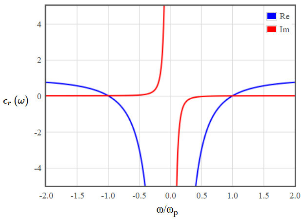   Figure 1: Dielectric function for a metal.

4. Draw the dielectric function for a semiconductor with a bandgap of 1 eV.

   The imaginary part describes the absorption and therefore must be zero up to about the band gap (because photons with energies below the band gap can not be absorbed). The frequency corresponding to the band gap of 1 eV is

   \begin{equation*} \omega = \frac{E}{\hbar} \approx 1.52\cdot 10^{15} \mathrm{rad/s}. \end{equation*}

   The real part must be finite and positive at $\omega = 0$ and should go to $1$ for $\omega\to\infty$. In between there are usually resonances.

   

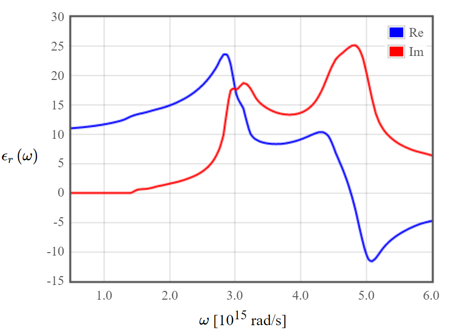   Figure 2: Dielectric function or a semiconductor with a bandgap of 1 eV.

5. Describe an experiment you could perform to determine the real and imaginary parts of the dielectric function of an insulator at $\boldsymbol{\omega = 0}$.

   At $\omega = 0 $ the imaginary part of the dielectric function is 0 (odd function!).

   You can use capacity measurements and from that you can calculate the dielectric constant ($\omega = 0$).

   \begin{equation*} C = \epsilon \frac{A}{d} \end{equation*}

6. Describe an experiment you could perform to determine the real and imaginary parts of the dielectric function of a metal at $\boldsymbol{\omega = 0}$.

   For a diffusive metal the dielectric function is given by

   \begin{equation*} \epsilon_r\left(\omega \right)=1+\chi_E=1-\frac{ne^2\tau}{m\omega \epsilon_0}\left(\frac{ \omega\tau+i}{1+\omega^2\tau^2} \right) = 1-\frac{ne^2\tau^2}{m \epsilon_0(1+\omega^2\tau^2)} + i\frac{1}{\omega(1+\omega^2\tau^2)}. \end{equation*}

   Thus for $\omega\to0$ the imaginary part diverges and the real part becomes

   \begin{equation*} \mathrm{Re}(\epsilon_r) = 1-\frac{ne^2\tau^2}{m \epsilon_0}. \end{equation*}

   The conductivity of a diffusive metal at low frequencies is

   \begin{equation*} \sigma = \frac{ne^2\tau}{m} \end{equation*}

   and these two equations can be combined to give

   \begin{equation*} \mathrm{Re}(\epsilon_r) = 1 - \frac{m\sigma^2}{ne^2\epsilon_0}. \end{equation*}

   Therefore the real part can easily be calculated from a conductivity measurement and the imaginary part diverges.

2. Dielectric function II (insulator)

1. Sketch the dielectric function of an insulator.
2. Draw the corresponding reflectance of light striking the normal to the surface from vacuum.
3. How can you calculate the dielectric function of an insulator from the electronic bandstructure?
4. How can you measure the dielectric function of an insulator at zero frequency?
5. How can you measure the dielectric function at optical frequencies?
6. How does the band gap of the insulator manifest itself in the dielectric function?
7. Sketch the real and imaginary parts of the dielectric function of an insulator.
8. What are the limiting values for the real and imaginary parts of the dielectric function at high frequency? Why?
9. The dielectric constant of materials used in a supercapacitor can be high ($\epsilon_r \sim 1000$). Explain why the dielectric constant is temperature dependent. The index of refraction $n = \mathrm{Re} [\sqrt{\epsilon_r]}$ is not so large for these materials ($n \sim 2$). Why is this so?

Solution

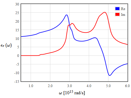
1. Sketch the dielectric function of an insulator.

   

   Figure 3: Dielectric function for an insulator (diamond).

2. Draw the corresponding reflectance of light striking the normal to the surface from vacuum.

   The reflection coefficient of light striking the crystal normal to the surface from vacuum ($\epsilon_r=1$) is,

   

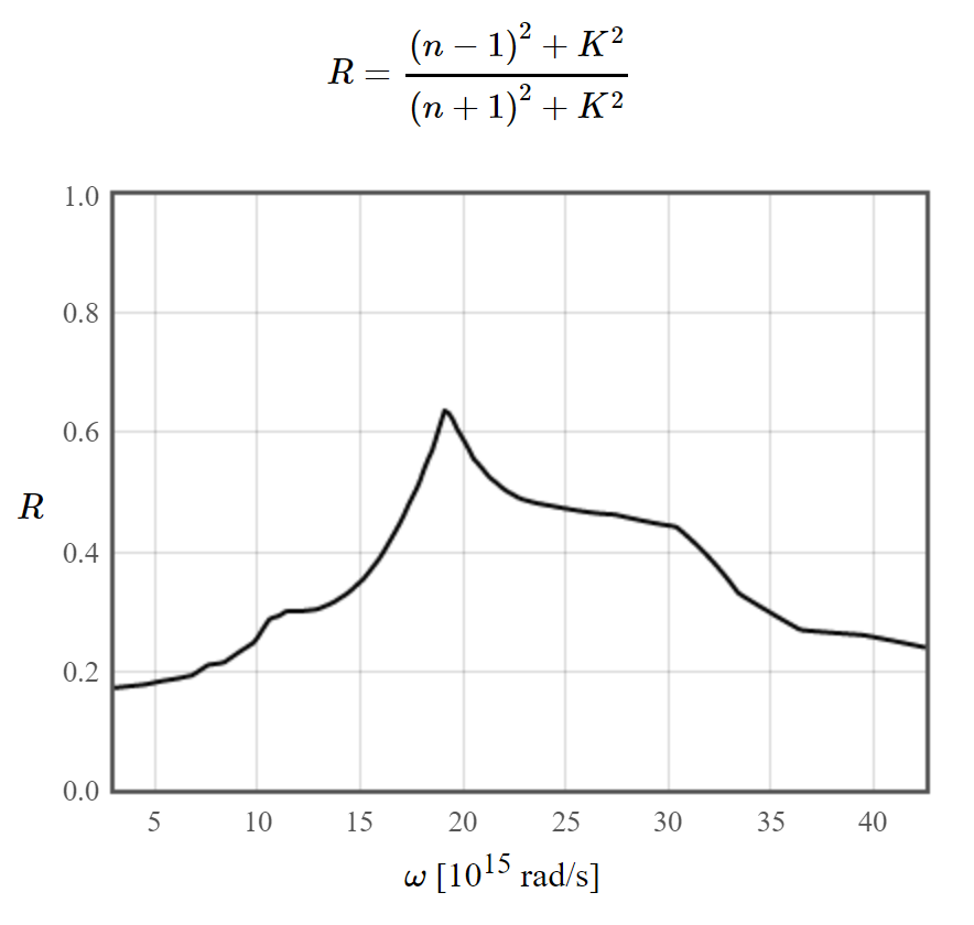   Figure 4: reflectance of light striking the normal to the surface from vacuum (diamond).

3. How can you calculate the dielectric function of an insulator from the electronic bandstructure?

   From the band structure (dispersion relation) you can calculate the optical absorption spectrum. The absorption rate is calculated using Fermi's golden rule for a transition from an occupied electron state into an empty state. The conservation of energy requires that the two electrons states have the same $\vec{k}$. The absorption coefficient is related to the extinction coefficient, which again is the imaginary part of the square root of the dielectric function. With the Kramer-Kronig relations you can calculate the real part of the square root of the dielectric function. To get the dielectric function you simply square the combined result.

   \begin{equation*} \alpha =\frac{2\omega K}{c} \end{equation*} \begin{equation*} \sqrt{\epsilon_r} = n +iK \end{equation*}

   $\alpha$ ... absorption coefficient, $c$ ... speed of light in the medium, $K$ ... extinction coefficient, $n$...index of refraction

4. How can you measure the dielectric function of an insulator at zero frequency?

   At $\omega = 0 $ the imaginary part of the dielectric function is 0 (odd function!).

   You can use capacity measurements and from that you can calculate the dielectric constant ($\omega = 0$).

   \begin{equation*} C = \epsilon \frac{A}{d} \end{equation*}

5. How can you measure the dielectric function at optical frequencies?

   Absorption and/or index of refraction measurement with subsequent determination of the dielectric function.

6. How does the band gap of the insulator manifest itself in the dielectric function?

   The imaginary part of the dielectric function is responsible for optical absorption. Since an insulator can not absorb photons with frequencies smaller than the band gap, the imaginary part of the dielectric function must be zero up to the frequency corresponding to the band gap.

   Besides, materials with bandgaps have no carriers at zero temperature. At finite temperature one can say that

   \begin{equation*} \epsilon \sim n \sim \exp\left(-\frac{E_g}{k_b T}\right). \end{equation*}

   This means that the larger the bandgap, the less free carriers, and the lower the dielectric constant.

7. What are the limiting values for the real and imaginary parts of the dielectric function at high frequency? Why?

   The imaginary part of the dielectric function goes to zero and the real part to a finite positive value $\epsilon_r(\infty)$.

   In fact the susceptibility must go to zero for $\omega\to\infty$ (thus $\epsilon_r\to1$), because the system can not respond to frequencies much higher than any resonance. However, there are often resonances at very high frequencies (for ionic crystals typically in the UV range), which are not taken into account, because they are outside the considered frequency range. Instead the existence of these high-frequency resonances is incorporated in the model by setting the susceptibility to a finite value for high frequencies.

   The imaginary part goes to zero basically for the same reason: Far from the resonance the system does not really react any more and therefore can not absorb energy from the fields.

8. The dielectric constant of materials used in a supercapacitor can be high ($\boldsymbol{\epsilon_r \sim 1000}$). Explain why the dielectric constant is temperature dependent. The index of refraction $\boldsymbol{n = \mathrm{Re} [\sqrt{\epsilon_r}]}$ is not so large for these materials ($\boldsymbol{n \sim 2}$). Why is this so?

   In materials with existing dipoles, which simply align with the external field, the situation is the same as in a paramagnet and the electric susceptibility follows a Curie-Weiss law

   \begin{equation*} \chi_E \propto \frac{1}{T}. \end{equation*}

   If the dipoles are induced by the external field, then the polarizability of the atoms can be temperature-dependent. Moreover, the polarization depends on the dipole density, which also changes with temperature.

   The dielectric constant for a capacitor is usually measured at $\omega = 0$. Since the refractive index is an optical property it is measured at high frequencies and the measured properties cannot be compared. Would it be measured at at $\omega = 0$ the refractive index would be $\sqrt{1000}$ because the imaginary part has to be zero and $\sqrt{\epsilon_r} = n + iK$.

   This is a typical behavior, because at high driving frequencies, which are far above all characteristic frequencies of the system, the system can not respond to the drive fast enough and the response is small.

3. Dielectric function III

The dielectric function of some material is shown in the following figure.

1. What properties does this material have? Note that the real part of the dielectric function is negative for some frequencies.
2. What are the limiting values of the real and imaginary parts of the dielectric function at $\omega=0$ and $\omega\to\infty$?
3. How is the dielectric function related to optical absorption measurements?
4. How is the dielectric function related to conductivity measurements at microwave frequencies?

Solution

1. What properties does this material have? Note that the real part of the dielectric function is negative for some frequencies.

   Due to the course of the illustration it should be a semiconductor. You can also see two resonance frequencies and up to the second one you have a (decaying) propagating solution ($\mathrm{Re}\, \epsilon_r(\omega)>0$). In the negative range ($\mathrm{Re}\,\epsilon_r(\omega)<0$), no propagating solution exists. Due to that the reflectivity is close to 1.

2. How is the dielectric function related to optical absorption measurements?

   The square root of the dielectric function is related to the extinction coefficient $K$ and the index of refraction $n$ via

   \begin{equation*} \sqrt{\epsilon} = n + iK. \end{equation*}

   The quantity $iK$ tells you how quickly the light is absorbed and $n$ how it is refracted. These are measurable quantities. The absorption coefficient is

   \begin{equation*} \alpha = \frac{2\omega K}{c}. \end{equation*}

   Due to that relation $\alpha$ can be calculated from the measurement of $K$. Since the real and imaginary part of the dielectric function are connected by the Kramers Kronig relations the whole dielectric function could in principle be calculated from the optical absorption.

3. How is the dielectric function related to conductivity measurements at microwave frequencies?

   \begin{equation*} \epsilon(\omega) = 1 + \chi = 1 + \frac{\sigma(\omega)}{i\omega \epsilon_0} \end{equation*}

   Below about 100 GHz the frequency dependent conductivity is normally used.

   Above about 100 GHz the dielectric function is used (optical experiments).

4. Ionic crystal

1. Sketch the dielectric function for this material. How could the Kramers-Kronig relation be used to check the form of the dielectric function?
2. Sketch the polariton dispersion relation for the ionic crystal. Use the same scale for the frequency axis as in part (a).
3. Sketch the reflectance for the ionic crystal for normally incident light. Use the same scale for the frequency axis as in part (a).
4. What are polarons? How could you measure the properties of polarons in this material?

Solution

1. Sketch the dielectric function for this material. How could the Kramers-Kronig relation be used to check the form of the dielectric function?

   With the Kramers-Kronig relationship, you can use the real part of the function to represent the imaginary part or vice versa. It should follow the same course as in the figure, but slight deviations may occur due to zero crossings (Cauchy Integral, Cauchy principle value - go around the singularity and take the limit as you pass by arbitrarily close).

   

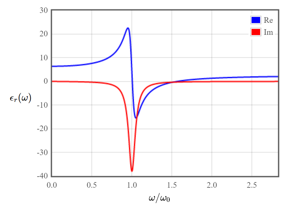   Figure 5: Dielectric function for an ionic crystal.

2. Sketch the polariton dispersion relation for the ionic crystal. Use the same scale for the frequency axis as in part (a).

   

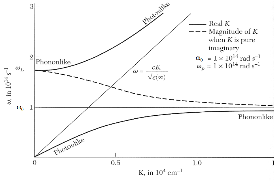   Figure 6: Polariton dispersion relation for the ionic crystal.

   The frequency $\omega_0$ in this plot corresponds to $\omega_0$ in the upper plot, which is indicated at ∼10¹⁴ rad/s.

3. Sketch the reflectance for the ionic crystal for normally incident light. Use the same scale for the frequency axis as in part (a).

   

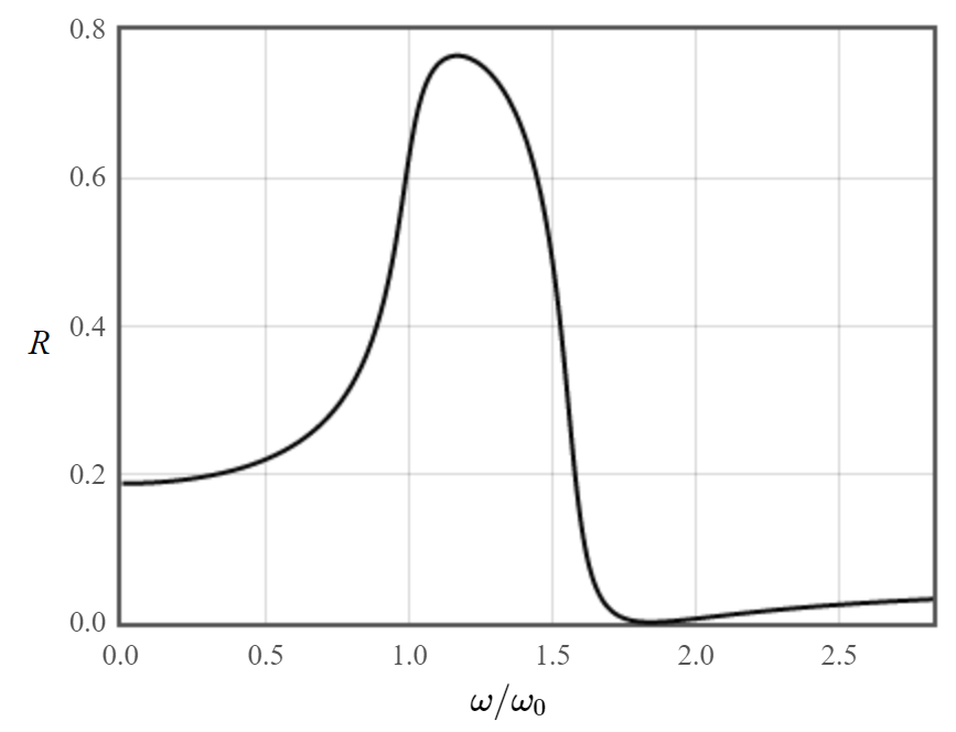   Figure 7: Reflectance for the ionic crystal for normally incident light..

   The frequency $\omega_0$ in this plot corresponds to $\omega_0$ in the upper plot, which is indicated at ∼10¹⁴ rad/s.

4. What are polarons? How could you measure the properties of polarons in this material?

   A polaron is a quasiparticle used in condensed matter physics to understand the interactions between electrons and atoms in a solid material.

   Briefly, polaron is the quasi-particle (i.e. a particle-like elementary excitation) of a system of electrons coupled with the lattice vibrations, or phonons. Considering for simplicity a system of independent electrons, in an ideal rigid periodic lattice electrons move unperturbed through the lattice in Bloch states. When the lattice is allowed to vibrate, with each atom oscillating around its average position, at any given instance the lattice is no longer in its ideal periodic form, resulting in the scattering of electrons from the Bloch states corresponding to the ideal rigid lattice. In turn, the movement of electrons through the lattice polarises the lattice, which like an assembly of electrons is polarisable. Taking account of this mutual interaction (electrons on phonons and phonons on electrons), the elementary excitations of the system are no longer describable in terms of a mere redistribution of electrons from the occupied Bloch states in the ground state into the unoccupied Bloch states, both corresponding to the rigid lattice.

   For measurement techniques and more details see question 5 in Quasiparticles.

5. Diffusive Metal I

1. What is the differential equation that describes the motion of an electron in a diffusive metal? (Newton’s law)
2. What is the impulse response function for a diffusive metal? Sketch the impulse response function
3. How is the impulse response function related to the dielectric function of a diffusive metal. Sketch the dielectric function for positive and negative frequencies.
4. How can you measure the dielectric function at DC and at optical frequencies?
5. How can you calculate the reflectivity of a diffusive metal from the impulse response function? Plot the reflectivity as a function of the frequency.
6. What determines the plasma frequency?

Solution

1. What is the differential equation that describes the motion of an electron in a diffusive metal? (Newton’s law)

   For high frequencies

   \begin{equation*} m\frac{dv(t)}{dt}+\frac{ev(t)}{\mu}=-eE(t). \end{equation*}

   For low frequencies $v(t)\approx \mu E(t)$.

2. What is the impulse response function for a diffusive metal? Sketch the impulse response function

   If the electric field is pulsed on for a short time, the driving force of the electric field can be described by a delta-function. Thus the solution of the differential equation is velocity of the electrons

   described by the impulse response function $g(t)$, that is sometimes called Green’s function.

   \begin{equation*} m\frac{dg(t)}{dt}+\frac{eg(t)}{\mu}=-e\delta(t). \end{equation*}

   Solving this equation, we get a exponential decaying solution for response of the velocity as a function of time. This is the impulse response function for a diffusive metal.

   \begin{equation*} g(t) = -\frac{e}{m} \exp{-\frac{et}{\mu m}} \end{equation*}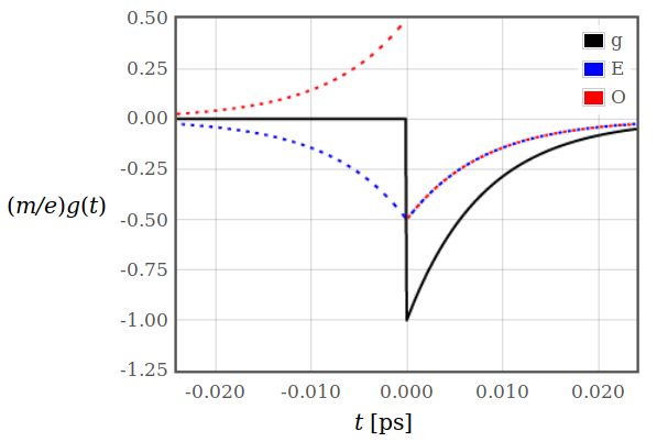
   

   Figure 8: Average electron velocity as a function of time if the electric field is pulsed on for a short time (impulse response function $g(t)$). The plot also shows the even and odd parts of the impulse response function.

   As we can see in figure 8, the electrons suddenly start moving when the electric field is pulsed on for a short time at $t = 0$, but the velocity decays to zero with a time constant $\tau = \frac{m\mu}{e}$.

   \begin{equation*} g(t) = -\frac{e}{m} \exp{-\frac{t}{\tau}} \end{equation*}

3. How is the impulse response function related to the dielectric function of a diffusive metal. Sketch the dielectric function for positive and negative frequencies.

   The impulse response function is the response of the system to a $\delta$-function excitation, which must be zero before the excitation (see above). The generalized susceptibility is the Fourier transform of the impulse response function and must obey the Kramers-Kronig relations (which relate real and imaginary part due to the causality restriction).

   The generalized susceptibility of a diffusive metal is defined by

   \begin{equation*} \chi\left(\omega \right)=\frac{v\left(\omega\right)}{E\left(\omega\right)} \end{equation*}

   and the electric susceptibility by

   \begin{equation*} \chi_E(\omega)=\frac{P\left(\omega\right)}{\epsilon_0 E\left(\omega\right)}=\frac{-ner\left(\omega\right)}{\epsilon_0 E\left(\omega\right)}=\frac{-nev\left(\omega\right)}{i\omega \epsilon_0 E\left(\omega\right)}. \end{equation*}

   Combining these equations relates the electric susceptibility to the generalized susceptibility:

   \begin{equation*} \chi_E(\omega) = -\frac{ne}{i\omega\epsilon_0}\chi(\omega) \end{equation*}

   and the dielectric function is simply $1+\chi_E$, thus

   \begin{equation*} \epsilon_r(\omega) = 1+\chi_E(\omega) = 1-\frac{ne}{i\omega\epsilon_0}\chi(\omega). \end{equation*}

   Hence the relation between the impulse response function $g(t)$ and the dielectric function $\epsilon_r(\omega)$ can be summarized as

   \begin{equation*} \epsilon_r(\omega) = 1+\chi_E(\omega) = 1-\frac{ne}{i\omega\epsilon_0}\mathcal{F}[g(t)]. \end{equation*}
   

   Figure 9: Real and imaginary part of the dielectric function of a diffusive metal as a function of $\omega$.

4. How can you measure the dielectric function at DC and at optical frequencies?

   With DC, the conductivity must be measured and then converted into the dielectric function (see question 1f).

   At optical frequencies: Absorption and index of refraction measurement with subsequent determination of the dielectric function from $\sqrt{\epsilon_r} = n + iK$.

5. How can you calculate the reflectivity of a diffusive metal from the impulse response function? Plot the reflectivity as a function of the frequency.

   Use the relations from above and calculate with it the reflectivity in terms of the impulse response function instead of the dielectric function.

   

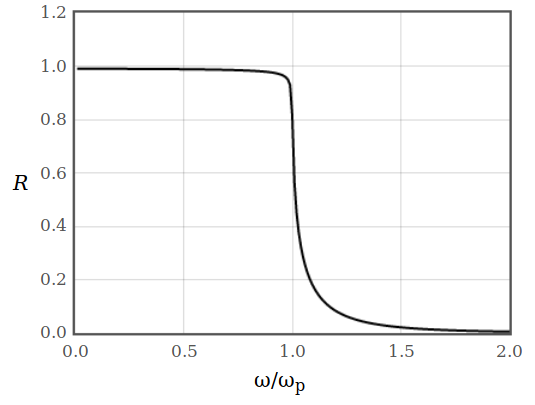   Figure 10: Reflectivity of a diffusive metal as a function of $\omega$.

   The reflectivity can also be drawn as a function of frequency. The equation for the reflectivity in terms of the dielectric function is

   \begin{equation*} R = \frac{(n-1)^2+K^2}{(n+1)^2+K^2}. \end{equation*}

   The index of refraction $n$ and the extinction coefficient $K$, that are used to calculate the reflectivity, can be obtained from the dielectric function. The refractive index is the real part and the extinction coefficient is the imaginary part of the square root of the dielectric function.

   

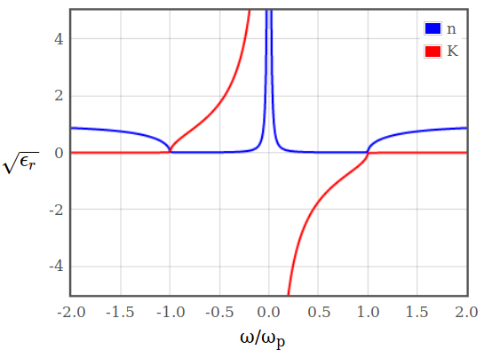   Figure 11: Index of refraction $n$ and extinction coefficient $K$ as a function of $\omega$.

6. What determines the plasma frequency?

   The plasma frequency is fully determined by the electron density $n$:

   \begin{equation*} \omega_p^2=\frac{ne^2}{m\epsilon_0}. \end{equation*}

6. Diffusive Metal II.

The differential equation that describes the motion of electrons in a diffusive metal is

1. Sketch the impulse response function that solves this equation.
2. Explain how you can derive the electrical conductivity from this equation.
3. We derived a frequency dependent conductivity using the dielectric function and a temperature dependent conductivity using the Boltzmann equation. How are these two quantities related? How are either of those solutions related to the differential equation above?

Solution

1. Sketch the impulse response function that solves this equation.

   If the electric field is pulsed on for a short time, the driving force of the electric field can be described by a delta-function. Thus the solution of the differential equation is velocity of the electrons

   described by the impulse response function $g(t)$, that is sometimes called Green’s function.

   \begin{equation*} m\frac{dg(t)}{dt}+\frac{eg(t)}{\mu}=-e\delta(t). \end{equation*}

   Solving this equation, we get a exponential decaying solution for response of the velocity as a function of time. This is the impulse response function for a diffusive metal.

   \begin{equation*} g(t) = -\frac{e}{m} \exp{-\frac{et}{\mu m}} \end{equation*}
   

   Figure 12: Impulse response function for a diffusive metal. In this plot the even and odd parts of the function are also shown.

2. Explain how you can derive the electrical conductivity from this equation.

   Rewrite the equation to

   \begin{equation*} m \frac{dv(t)}{dt}+ \frac{ev(t)}{\mu}=-eE(t) \end{equation*}

   and assume a harmonic solution $E(\omega)e^{i\omega t}, v(\omega)e^{i\omega t}$$\Rightarrow$

   \begin{equation*} \left( -\frac{ i\omega m}{e}-\frac{1}{\mu}\right)v(\omega)=E(\omega) \end{equation*} \begin{equation*} \frac{v(\omega)}{E(\omega)}=\left( -\frac{ i\omega m}{e}-\frac{1}{\mu}\right)^{-1}=-\mu(1+i\omega \tau)^{-1} = \frac{-\mu(1-i\omega\tau)}{1+\omega^2\tau^2} \end{equation*} \begin{equation*} \sigma(\omega)=\frac{j(\omega)}{E(\omega)}=-ne\frac{v(\omega)}{E(\omega)}=ne\mu\left( \frac{1-i\omega\tau}{1+\omega^2\tau^2}\right) \quad\text{with}\quad \tau=\frac{\mu m}{e} \end{equation*} \begin{equation*} \sigma(\text{low } \omega)\approx ne\mu ,\qquad \sigma(\text{high } \omega)\approx-\frac{ine^2}{\omega m} \end{equation*}

   The next two equations are an addition

   \begin{equation*} \chi(\omega)= \frac{\sigma(\omega)}{i\omega\epsilon_0} \end{equation*} \begin{equation*} \epsilon(\omega)=1+\chi=1+\frac{\sigma(\omega)}{i\omega\epsilon_0} \end{equation*}

   This means that it is possible to describe the motion of an electron in a metal as well as in an insulator by both, the dielectric function and the electric conductivity. Though it is convention to use the conductivity for frequencies below about 100 GHz and the dielectric function above about 100 GHz, especially since we are usually dealing with optical experiments in that region.

3. We derived a frequency dependent conductivity using the dielectric function and a temperature dependent conductivity using the Boltzmann equation. How are these two quantities related? How are either of those solutions related to the differential equation above?

   They are only related for low temperatures and low frequencies. In these limits both derivations yield the same result.

   The dielectric function and therefore the frequency-dependent conductivity can be obtained from the equation above via some additional relations.

   The temperature dependent conductivity cannot be derived directly from this equation, the Boltzmann equation and the basic definition of electrical current have to be used instead.

7. Plasma frequency

1. The specific heat of a metal is measured at low temperatures to have the form, $c_V= \gamma T$, where T is the absolute temperature. How could this information be used to determine the plasma frequency of the metal?
2. How could the plasma frequency be measured?
3. De Haas-van Alphen oscillations are measured for a metal. How could you tell from these measurements if the states at the Fermi surface are electron-like or hole-like?
4. Use the form of the dielectric function to explain why losses increase with frequency in the microwave regime.

Solution

1. The specific heat of a metal is measured at low temperatures to have the form, $\boldsymbol{c_V= \gamma T}$, where T is the absolute temperature. How could this information be used to determine the plasma frequency of the metal?

   The plasma frequency of a metal only depends on its electron density:

   \begin{equation*} \omega_p^2 = \frac{ne^2}{m\epsilon_0}. \end{equation*}

   For low temperatures the electron contribution to the specific heat dominates over the phonon contribution and the specific heat of a free electron gas only depends on the electron density and temperature via

   \begin{equation*} c_V \approx \frac{\left(3\pi^2n\right)^{1/3}m^*}{3\hbar^2}k_B^2T. \end{equation*}

   Hence, the electron density can be calculated from the proportionality constant $\gamma$ and the plasma frequency from the electron density.

2. How could the plasma frequency be measured?

   The plasma frequency can be determined from an EELS (electron energy loss spectroscopy) measurement. In this measurement the energy loss of electrons is measured after passing through the sample. If these electrons excite plasmons in the material, then their energy loss must be an integer multiple of the plasma frequency. Therefore the plasma frequency is simply the distance between adjacent peaks in the EELS measurement.

3. De Haas-van Alphen oscillations are measured for a metal. How could you tell from these measurements if the states at the Fermi surface are electron-like or hole-like?

   The de Haas-van Alphen oscillations do not depend on the type of charge carriers, for both electrons and holes the formula

   \begin{equation*} S\left(\frac{1}{B_{n+1}}-\frac{1}{B_n}\right) = \frac{2\pi e}{\hbar^2} \end{equation*}

   is valid, where $S$ is the cross-section of the Fermi surface. From multiple de Haas-van Alphen measurements in various directions in principle the whole Fermi surface can be constructed and from its shape the type of charge carriers could somehow be determined.

   However, to distinguish electron-like and hole-like orbits, Hall effect measurements are much better suited, because the Hall coefficient has opposite sign for electrons and holes.

4. Use the form of the dielectric function to explain why losses increase with frequency in the microwave regime.

   For metals the dielectric function has the form

   \begin{equation*} \epsilon_r\left(\omega \right)=1-\frac{ne\mu}{\omega \epsilon_0}\left(\frac{ \omega\tau+i}{1+\omega^2\tau^2} \right). \end{equation*}

   In the microwave regime $\omega\tau \ll 1$ and the quadratic term in the denominator can be neglected, leading to

   \begin{equation*} \epsilon_r\left(\omega \right) \approx 1-\frac{ne\mu\tau}{\epsilon_0} - i\frac{ne\mu}{\omega\epsilon_0}. \end{equation*}

   The extinction coefficient $K$ can be determined from

   \begin{equation*} \sqrt{\epsilon_r} = n + iK \implies \epsilon_r = n^2-K^2 + 2inK. \end{equation*}

   For the low frequency limit above this means

   \begin{equation*} n^2-K^2 \approx const. \quad\text{and}\quad nK \propto \frac{1}{\omega}. \end{equation*}

   From the first relation it is clear that $n$ and $K$ must have the same frequency dependence, thus

   \begin{equation*} K \propto \frac{1}{\sqrt{\omega}}. \end{equation*}

   In terms of $K$ the absorption coefficient is given by

   \begin{equation*} \alpha = \frac{2\omega K}{c} \propto \sqrt{\omega}, \end{equation*}

   hence in the low frequency range the absorption increases with increasing frequency. Figure 13 shows the absorption coefficient of a diffusive metal at low frequencies in the microwave range.

   

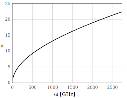   Figure 13: Absorption coefficient of a diffusive metal in the low frequency range.

   In the case of a dielectric, the imaginary part grows continuously up to the frequency of the first resonance and therefore also the absorption increases with frequency.