The electrical resistance of a material represents the opposition to the flow of current. For most scenarios, Ohm's law $V=R·I$ using a constant resistance $R$ is enough to describe a voltage-current dependence.
However, resistance is actually proportional to the mobility of carriers in a material, and this results to be heavily affected by temperature.
At normal temperature range, raising $T$ induces phonon scatering, reducing the mobility and therefore resistance.
In this lab experience, several measurements were performed on a thin stainless steel wire, with the objective of observing its resistance dependence with temperature.
Equipment Used
Sourcemeter
For the voltage supply and for the electrical measurements the Keithley 2636A Series Sourcemeter was used.
This sourcemeter has two separate channels.
To communicate with the wire, already existing python scripts were used and slightly edited.
The example python scripts as well as the Keithley 2600 Pyhton library can be found here:
Diode Measurements with a Sourcemeter.
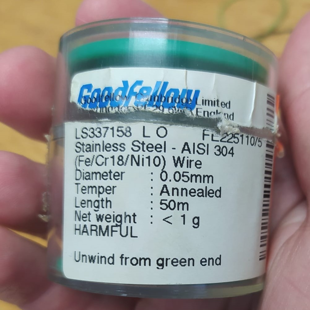
Steel wire
The measurements for the temperature dependent resistance of a metal were done on a stainless steel [AISI 304 (Fe/Cr18/Ni10)] wire.
Its length was not accurately measured, but it is expected to be around L = 10 cm.
Fig.1: Stainless steel wire
Climate Chamber
To determine a more precise resistance-temperature behavior, the following Vötsch VT4002 climate chamber was employed, allowing the wire to stay at a certain temperature while measuring resistance.
Experimental Setup and Measurements
Temperature dependent electrical resistance of a metal
To measure the electrical characteristics of the iron wire, it was wrapped around two thicker wires which were than connected to the breadboard
with a clamp. The setup can be seen on Fig.2 and since the wire can not be seen well on the picture, the connecting points are marked with
red arrows.
Fig.2: Experimental setup
The next step was to sweep the voltage and measure the current through the wire. To do this, following python script was used:
However, using this script, the measurement directly starts at the low starting voltage and increases in time. As discussed in the results, this affects
the measurements unintentionally. Therefore the script was edited, so that the voltage starts at 0 V, increases to the positive voltage
limit, decreases to the negative voltage limit and than again increases to 0 V. Since we did not fully know how much power the wire would stand
before breaking, we started the measurement at a very small voltage range of [-0.04,0.04] V, increased the range with each measurement and
eventually reached a range of [-20,20] V.
Climate Chamber for the wire
The next step was to measure the relation between the temperature of the wire an its resistance, this was done with the help of the climate chamber. The sweep was done between 5ºC and 60ºC with the following code:
Results and Discussion
Voltage-Intensity measurement
Fig.3 shows the measurement when directly sweeping from negative voltage to positive voltage. At first voltages, one can see an a sudden jump in the current which is not expected.
This behavior was not consistent and appeared for different starting voltages. This happened as a consequence of measurements directly starting at low voltages where the wire was not heated yet.
But as the following measurements show, the resistance increases with rising temperature.
Fig.3: Intensity versus voltage on the wire
The results of the voltage sweep are shown in Fig 4. For this measurement the modified python script was used, measurements start
at 0 V, reach 20 V, then are lowered to -20 V and end in the starting point. This explains the hysteresis like behavior of the curve.
Fig.4: Intensity versus voltage on the wire
As it can be observed, the actual behavior differs from the linear relation predicted by Ohm's law for higher voltages. Since
the wire is thin, it heats up easily with higher power submitted. This heating causes an increase in the resistance, curving down the instensity according to
$$
I=\frac{V}{R(T)}
$$
The values have been measured also in a negative range so the symmetry can be observed.
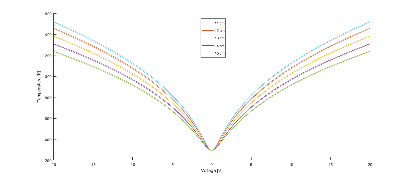
An attempt of predicting the temperature of the wire as the voltage is increased can be done. In order to do so, Stefan-Boltzmann law can be used,
as the power submitted to the wire is being radiated. For this it is assumed for the wire to behave like a black body.
$$
P=S \sigma \left(T^4-T_0^4\right)
$$
Where $P$ is the power emitted, $S$ the radiating surface and $\sigma$ the Stefan-Boltzmann constant. The power at laboratory temperature $T_0$ must be substracted so only the increment caused
by the current is being accounted. It will be set to 292K. Since the power can be expressed as $IV$ and the surface is cilindrical, one finds $S=2\pi r l$ where $r$ is the radius and $l$ the length of the wire.
With this,
$$
T=\left(\frac{IV}{2 \pi r l \sigma}+T_0^4\right)^{1/4}
$$
The results of this calculation are shown in Fig. 3. Since the length of the wire was not accurately measured, a sweep varying slightly $l$ has been carried out.
Fig.5: Stefan-Boltzmann calculated temperatures for slightly different lengths of the wire
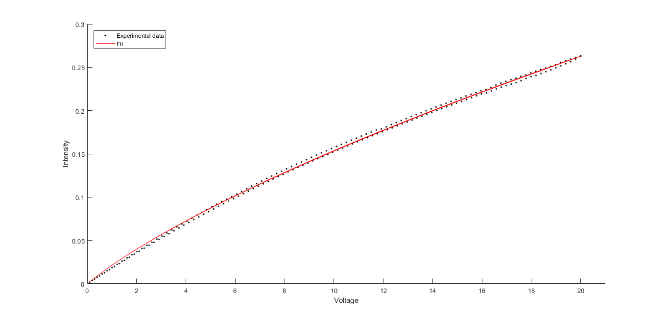
Now using these obtained values, a fit can be made to check if the temperatures actually describe the experimental curve.
For this sake, expanding the resistance up to a linear term, one finds
$$
R(T) \approx R_0+R_1 T
$$
Where $R_0$ and $R_1$ can be treated as fitting constants. This way, a good correlating fit ($r^2=0.9991$) is observed,
obtaining the values $R_0=34.92 \: \Omega$ and $R_1=0.0314 \: \Omega K^{-1}$. The best fitting value for the length of the wire showed to be $l=14 cm$. A comparison of the experimental data and the fit is showed in Fig.6 . Only the positive branch is shown for simplicity reasons.
Fig.6: Fit of the positive branch using calculated temperatures for $l=14 cm$
Resistance dependence of the wire
The results obtained from the climate chamber experiment were not very clear. First of all, an increase in the resistance for higher temperature values was expected to happen, as we can see in the following data, this was not the case. Also, the code ran for several times but there was a problem with it that stop the climate chamber for going to the end. The best data obtained is shown below:
Therefore, due to not having conclusions from this last part, we encourage the next students to work on it.