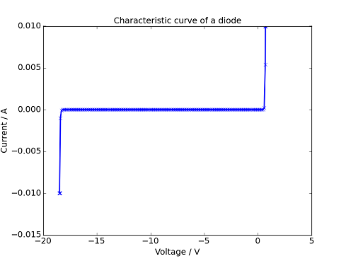
Diode Measurements with a Sourcemeter

This page describes how to use a Keithley 2600 Series Sourcemeter to measure the current-voltage characteristics of a diode. The sourcemeter consists of two source-measurement units (SMUs). Each SMU can source a voltage and measure a current or source a current and measure a voltage. Connect one side of the diode to the Hi terminal of an SMU and the other side to a Lo terminal of the same SMU. We will use a Python program to execute a loop where in each step of the loop the sourcemeter will source a voltage across the diode and then measure the current through the diode. The data that is collected will then be plotted using the package matplotlib.

A diode is a two-terminal electrical device that lets current pass in one directly much more easily than in the other direction. It typically consists of a single crystal of a semiconductor that has p-doping on one side and n-doping on the other side. Positively charged holes are mobile on the p-side and negatively charged electrons are mobile on the n-side. If a positive voltage is applied to the p-side and a negative voltage is applied to the n-side, the electrons and holes will be pushed towards each other and the electrons will fall into the holes. This is forward bias. If a positive voltage is applied to the n-side and a negative voltage is applied to the p-side, the electrons and holes will be pulled away from each other. This is reverse bias.

Download the Python script example_diode.py and the Python library Keithley 2600 Python library and save them in your directory.

from KeithleyV15 import SMU26xx
import matplotlib.pyplot as plt

"""
EXAMPLE: characteristic curve of a diode

Schematic:

--------------
    |            |
  -----         -|-
  | A | SMU     \|/
  -----         -|-
    |            |
    --------------

"""

""" ******* Connect to the Sourcemeter ******** """

# initialize the Sourcemeter and connect to it
# you may need to change the IP address depending on which sourcemeter you are using
sm = SMU26xx("TCPIP0::129.27.158.189::inst0::INSTR")

# get one channel of the Sourcemeter (we only need one for this measurement)
smu = sm.get_channel(sm.CHANNEL_A)

""" ******* Configure the SMU Channel A ******** """

# reset to default settings
smu.reset()
# setup the operation mode
smu.set_mode_voltage_source()
# set the voltage and current parameters
smu.set_voltage_range(20)
smu.set_voltage_limit(20)
smu.set_voltage(0)
smu.set_current_range(0.05) #50 mA
smu.set_current_limit(0.05)
smu.set_current(0)

""" ******* Make a voltage-sweep and do some measurements ******** """

# define sweep parameters
sweep_start = -20
sweep_end = 20
sweep_step = 0.1
steps = int((sweep_end - sweep_start) / sweep_step)

# define variables we store the measurement in
data_current = []
data_voltage = []

# enable the output
smu.enable_output()

# step through the voltages and get the values from the device
for nr in range(steps):
    # calculate the new voltage we want to set
    voltage_to_set = sweep_start + (sweep_step * nr)
    # set the new voltage to the SMU
    smu.set_voltage(voltage_to_set)
    # get current and voltage from the SMU and append it to the list so we can plot it later
    [current, voltage] = smu.measure_current_and_voltage()
    data_voltage.append(voltage)
    data_current.append(current)
    print(str(voltage)+' V; '+str(current)+' A')

# disable the output
smu.disable_output()

# properly disconnect from the device
sm.disconnect()

""" ******* Plot the Data we obtained ******** """

plt.plot(data_voltage, data_current,'x-', linewidth=2)

# set labels and a title
plt.xlabel('Voltage / V', fontsize=14)
plt.ylabel('Current / A', fontsize=14)
plt.title('Characteristic curve of a diode', fontsize=14)
plt.tick_params(labelsize = 14)
plt.show()

example_diode.py

In the script, example_diode.py, first the source meter is initialized and then the voltage and current limits are set. Read the data sheet of the diode you are measuring to find out what currents and voltages it can tolerate. For the example measurements we used a BZY97C18 Zener diode. In the BZY97C18 data sheet it specifies that the diode can tolerate a maximum current of 66 mA.

A For-loop is defined in the script which sets the voltage across the diode using the 'smu.set_voltage()' command and then the voltage across the diode and the current through the diode are measured with the 'smu.measure_current_and_voltage()' command. Review the script and then run it. It should print out the datapoints and make a plot. An example current-voltage characteristic for a BZY97C18 Zener diode is shown below. There is a sharp increase in the current for forward bias voltages and an abrupt breakdown at -18.2 V in reverse bias.

The code steps the voltage from -20 V to +20 V but the sourcemeter will not apply a voltage that will cause the current to be higher than the current limit that was set.

For analysis later, it would be convenient to save the data. We will add some code that automatically saves the data in a text file and automatically transfers the data and the measurement script to ElabFTW (as TU Graz or KFU Graz student, you have an account). This code appends the time to the file name so that each measurment is saved in a separate file. Make a new directory and download the file 'example_diode2.py' into it. Download the library eLabFTW_config_api2_semilab.py, place it in your directory, and quickly adjust the library to your token as described here. Copy the Keithley 2600 Python library into this directory as well. Open the file, 'example_diode2.py' and find the line where the file names are defined and replace (your directory) with the name of the directory where the files should be saved.

from KeithleyV15 import SMU26xx
import matplotlib.pyplot as plt
import time
import datetime
import csv
import numpy as np

#libraries to handle ElabFTW
import os
import elabapi_python
from elabapi_python.rest import ApiException

"""
EXAMPLE: characteristic curve of a diode

Schematic:

--------------
    |            |
  -----         -|-
  | A | SMU     \|/
  -----         -|-
    |            |
    --------------

"""
# Connect to eLab and create an experiment
# Connect to eLab and create an experiment
experiment_title = "Diode Measurements"
elab_manager = eLab.Helper_elabftw()
experiment_ID = elab_manager.set_experiment(experiment_title)

""" ******* Connect to the Sourcemeter ******** """

# initialize the Sourcemeter and connect to it
# you may need to change the IP address depending on which sourcemeter you are using
sm = SMU26xx("TCPIP0::129.27.158.189::inst0::INSTR")

# get one channel of the Sourcemeter (we only need one for this measurement)
smu = sm.get_channel(sm.CHANNEL_A)

""" ******* Configure the SMU Channel A ******** """

""" ******* For saving the data ******** """

# Create unique filenames for saving the data
time_for_name = datetime.datetime.now().strftime("%Y_%m_%d_%H%M%S")
filename_csv = 'Diode' + time_for_name +'.csv'
filename_pdf = 'Diode' + time_for_name +'.pdf'

# Header for csv
with open(filename_csv, 'a') as csvfile:
        writer = csv.writer(csvfile, delimiter=';',  lineterminator='\n')
        writer.writerow(["Voltage / V", "Current / A"])

""" ******* Make a voltage-sweep and do some measurements ******** """

# define sweep parameters
sweep_start = -20
sweep_end = 20
sweep_step = 0.1
steps = int((sweep_end - sweep_start) / sweep_step)

# define variables we store the measurement in
data_current = []
data_voltage = []

# enable the output
smu.enable_output()

# disable the output
smu.disable_output()

# properly disconnect from the device
sm.disconnect()

""" ******* Plot the Data we obtained ******** """

plt.plot(data_voltage, data_current,'x-', linewidth=2)

# Upload files to eLab
# (1) store name of current script, necessary for upload
filename_scr = __file__

# (2) consider all data files that were generated
elab_manager.upload_file(experiment_ID, filename_csv)
elab_manager.upload_file(experiment_ID, filename_pdf)
elab_manager.upload_file(experiment_ID, filename_scr)

# as a final step show figure
plt.show()

example_diode2.py

There are three interesting regimes of this diode curve.

The forward bias regime where the current increases exponentially with current.
The reverse blocking regime where very little current flows.
The reverse breakdown regime where diode abruptly conducts in reverse bias.

Forward bias regime
In the forward bias regime we expect that the current to obey the diode formula,

$$I = I_S\left(\exp\left(\frac{eV}{\eta k_BT}\right) - 1\right)\hspace{0.5cm}\text{[A]}.$$

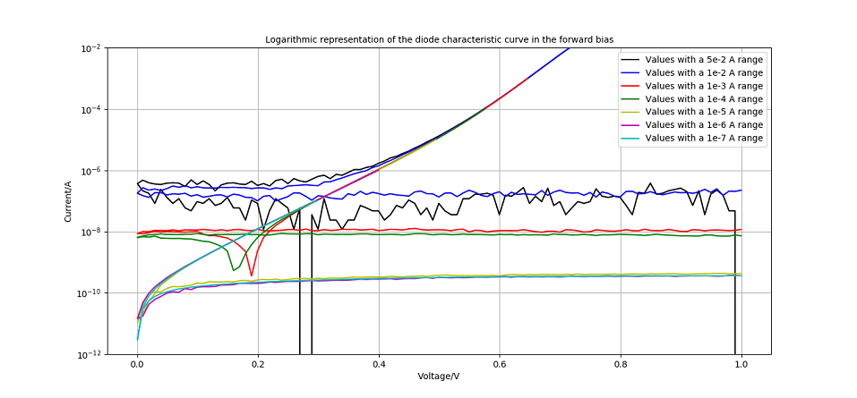
Here $I$ is the current, $I_S$ is the saturation current, $e$ is the elementary charge, $V$ is the voltage, $k_B$ is Boltzmann's constant, $T$ is the absolute temperature, and $\eta$ is the non-ideality factor which is usually between 1 and 2.

In the forward bias regime it is common to plot the logarithm of the current vs. voltage. Save the Python script with a different name and modify it to sweep the voltage from -1 V to 1 V. The sweep_step should be decreased to about 0.01 so that enough data is collected in this voltage range. Make a semilogarithmic plot $\log (I) $ vs. $|V|$ as shown below.

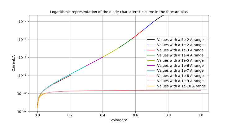
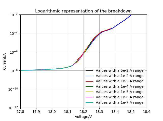
For larger positive voltages, the plot should be a straight line where the slope is $\frac{e}{\eta k_BT}$ and the intercept is $\log (I_S) $. It will be necessary to record the data for different current ranges. A current range of 100 mA will not measure the small currents near $V=0$ accurately. Below is a plot of $\log (I) $ vs. $V$ for different current ranges. Note that the larger current ranges give inacurate reading for low currents.

A program that reads the csv data files and plots $\log (I)$ vs. $V$ to make a plot like this is shown below.

plot_log.py

You can adjust the plot ranges to exclude the data that is taken where the current range is set poorly. An example of an adjusted plot is shown below.

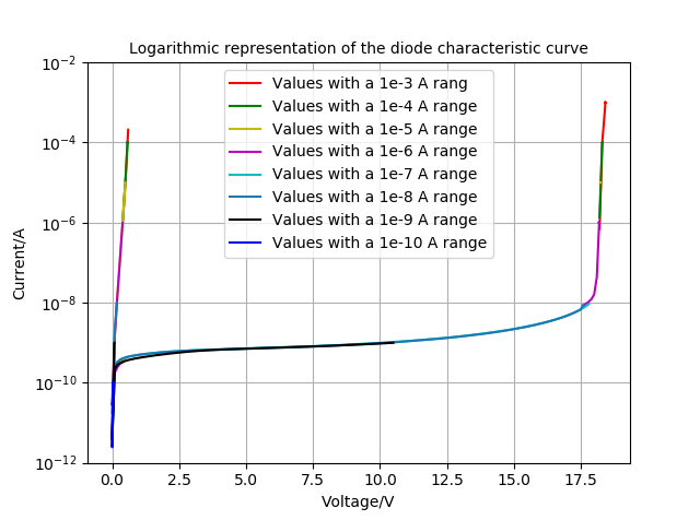
A plot of $\log (I) $ vs. $|V|$ over a wider voltage range that included the breakdown voltage is shown below.

Focusing on the region near breakdown shows a distinct change in the behavior of the current at $V=18.3\,\text{V}$.







Semiconductor Laboratory