Frequency dependent impedance measurements with the Stanford 830 lock-in amplifier

In order to measure the impedance of different electronic compounds the Stanford 830 lock-in amplifier is used. Lock-in amplifiers are used to extract signals with known carrier frequencies in noisy environments, therefore they are mostly used to measure the amplitude and the phase of an oscillating signal when the signal to noise ratio is very low. A short video that discusses the principles and applications of lock-in amplifiers in general can be found here.
The Stanford 830 lock-in amplifier has an integrated sinusoidal voltage source that generates the carrier wave and is directly connected to one side of the device under test (via the 'SINE OUT' connector). The other side of the electrical compound is connected to the signal input of the lock-in amplifier which is labeled by 'A/I'. For more information concerning the setup of the lock-in amplifier (configuration of inputs, setting of time constants etc.) see the webpage Frequency dependent impedance measurements from the course "Semiconductor Laboratory".

The impedance measurements were performed using the following electronic compounds:

• Resistors (1 M$\Omega$ and 100 M$\Omega$)
• Capacitors (22 pF and 100 pF)
• BNC cabels (with lengths of 160 cm and 465 cm)

The results of the measurements are displayed below.

The following Python script was used to conduct all measurements described in order to measure the impedance of the electrical compounds and the phase. The parameters in the script can be altered for different samples, for example the frequency range or the amplitude of the sine wave can be changed if necessary.
For the program to be executed, the StanfordResearchSystems Library has to be stored in the same folder as this Python script.

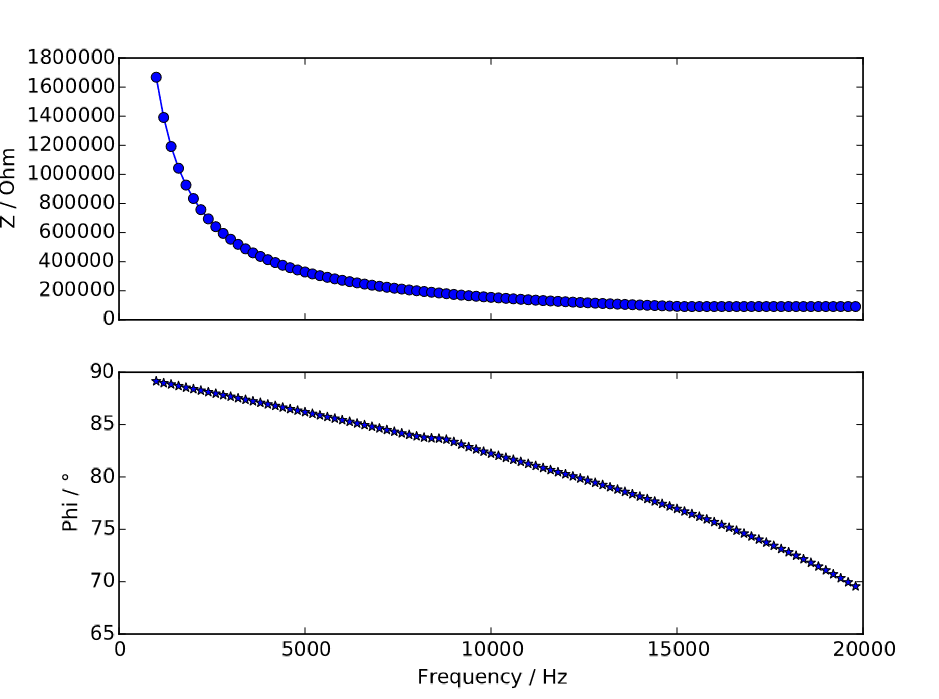
Using this program and modifying it whenever neccessary, the following results were obtained and afterwards fitted with Matlab.

The Python script not only generates a pdf-file with the plots, it also saves the data in a csv-file. The following box contains the data for the plots above (C = 100 pF).

The same measurement was repeated for a capacitor with a nominal capacitance of 22 pF. The data was fitted with Matlab according to the equation of the impedance of the series RLC circuit ($Z_{RLC} = \sqrt{R^2 + (X_L -X_C)^2} = \sqrt{R^2 + (\omega L - \frac{1}{\omega C})^2}$) and is plotted below together with the data and the fit for the capacitor with a nominal capacitance of 100 pF. The values in the legend are the results of the fits for the capacitances.

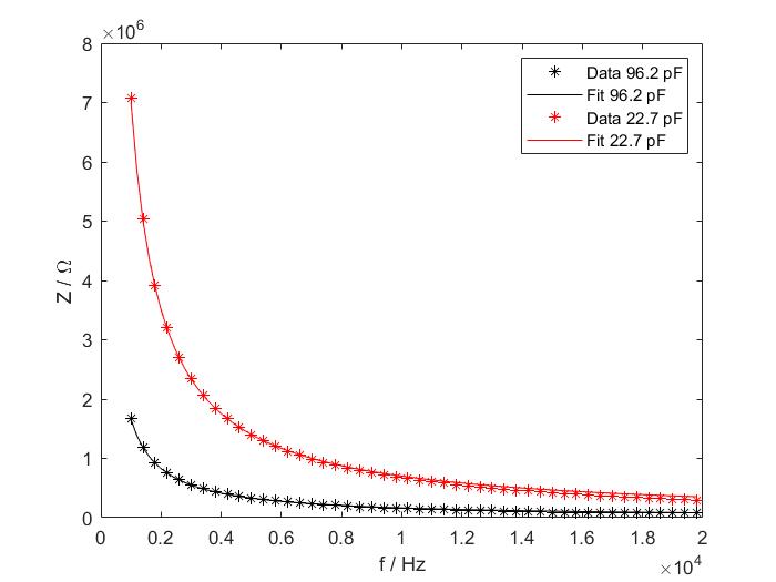
The box below contains the measured data for the capacitor with a nominal capacitance of 22 pF.

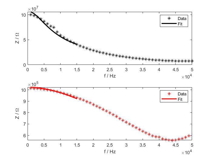
The results of the impedance measurement for two resistors with nominal resistances of 1 M$\Omega$ and 100 M$\Omega$ are shown in the figure below. The box below the figure contains the measured data for both resistors.
The measured values of the impedance at a frequency of 0 Hz are the resistances because there $X_C^{-1}$ is zero.
Because there is a parasitic capacitance of the wire parallel to the resistor, a fit of the measured data according to the impedance of a resistor parallel to a capacitor has been performed.
The impedance of a resistor parallel to a capacitor is given by $Z_{R||C} = \sqrt{\frac{1}{R^2} + (\omega C)^2}^{-1}$. There is also a parasitc inductance because of the wire, which is significantly smaller than the parasitc capacitance at low frequencies and is therefore not considered in the fit (fit extends up to a frequency of 15 kHz).
The results of the fits are:

• R = 107132535 $\Omega$, C = 2.4$\cdot 10^{-13}$ F
• R = 1023282 $\Omega$, C = 5.0$\cdot 10^{-12}$ F

The same impedance measurements were done with just BNC cables with lengths of 160 cm and 465 cm. The results were fitted afterwards to the impedance of an RLC series circuit. The cables connected the voltage output (wave generator) to the box that would contain the electrical component and after the box, the second cable was connected to the input of the lock-in amplifier. The results of the impedance measurements and the fits are shown in the figure below.
The results of the fits are

• cable length of 160 cm: R = 44.3 k$\Omega$, L = 0.35 H, C = 46.5 pF.
• cable length of 465 cm: R = 44.3 k$\Omega$, L = 0.81 H, C = 46.3 pF.

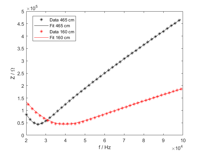
The box below contains the data for the cables with lengths of 160 cm and 465 cm. The frequency range for the shorter cable was chosen to start at 1 kHz, but the results in the figure are only shown starting at 20 kHz.

• Include lower as well as higher frequencies for the impedance measurements (also very small frequencies are possible).
• Measure the impedance of BNC cables with different lengths (without any other components), but connect the wave generator to the input of the lock-in amplifier using just one cable (without the box that normally contains the devices under test).
• Measure and fit the impedance of a parallel and/or serial RLC-circuit with known nominal characteristic values (resistance, capacitance and inductance) and compare the results from the fit with their nominal values.