Errors: general considerations

Processing math: 100%







Numerical Methods

Outline

Introduction
- Basics
- Errors
- Methodological and roundoff errors

Errors: general considerations

In numerical mathematics, input data is given to an algorithm which then produces output data. The algorithm is a finite number of precise instructions, which require specific input data and, executed in a given sequence, determine the output data. Typically, there are errors in the input data either because the input data is not known precisely or because it cannot be expressed precisely as finite-digit numbers. The algorithm typically introduces more errors. These errors can be methological errors or round-off errors associated with representing the state of the system at every step by finite-digit numbers. When working with a computer, it is of outmost importance to keep track of all possible errors so that the precision of the results that are obtained can be estimated. More discussion on errors in numerical methods can be found in references [Dorn, 1972] and [Björck, 1972 ].

Absolute and relative errors. Machine precision

Before discussing the various types of errors in more detail, it is useful to introduce the concept of absolute and relative error:

If $x$ is the (unknown) real value of a quantity and $\overline{x}$ is the relative approximate value obtained with a numerical calculation, we define:

$\begin{equation} \label{abs_err} \epsilon_a = x-\overline{x} \end{equation}$

absolute error and

$\begin{equation} \label{eq:rel_err} \epsilon_r = \frac{\epsilon_a}{\overline{x}}=\frac{x-\overline{x}}{\overline{x}} \end{equation}$

relative error of $\overline{x}$ .

In practical cases, it is usually preferrable to employ the relative error, given by formula $\ref{eq:rel_err}$ . The reason is clearly illustrated by the following simple example:

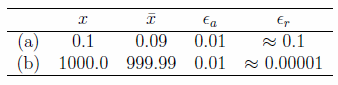
It is immediately clear that the approximation in (b) is much more satisfactory than in (a), although the absolute error is the same in both cases.

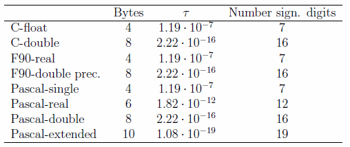
Another fundamental concept is that of machine precision: this is the smallest (positive) number $\tau$ , for which:

$\begin{equation} \nonumber 1+\tau >1 \end{equation}$

For a (non-existing) supercomputer that can save real numbers with arbitrary accuracy, the above inequality would be satisfied for all values of $\tau$ . In real computers, however, $\tau$ has a finite value, which it is very important to know. It can be estimated in practice using the algorithm shown in code block below.

<script> var tau,wold,wnew; tau = 1; wold = 1; do { tau = tau/2; wnew = wold+tau; } while (wnew != wold ); document.write("τ = "+2*tau+"<br />"); </script>
tau.cpp tau.f90

In this example, the equivalent code in c++ and FORTRAN is provided. To use this code it must be copied into a program that can execute it. Only JavaScript will execute in the webpage.

The results of the machine precision check algorithm obtained on a PC IBM are shown in the table below.

Input errors. Ill-conditioned problems

Input errors (i.e. inherent errors) are uncertainities in the input data with which the computer performs the calculation. These uncertainities can have several origins, i.e. experimental measuring errors, or roundoff errors.

If the results of a calculation are strongly influenced by this input errors we speak of an "ill-conditioned problem".

As an example of an ill-conditioned linear set of equations, we consider the example in [Dorn,1972], page 97:

$\begin{equation} x + 5.0y = 17.0 \end{equation}$

$\begin{equation} 1.5x + 7.501y = a \end{equation}$

We assume that $a$ is determined by an experiment, and thus affected by uncertainity:

$\begin{equation} a=25.503 \pm 0.001 \quad \end{equation}$

It is easy to verify that the exact solutions for this system for $a=25.503$ are: $x=2.0$ and $y=3.0$ .

The table below shows how the values of $x$ and $y$ change, if we assume that the last digit of $a$ changes by one unit:

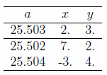
Obviously, this set of equations constitutes an extremely ill-conditioned problem! The results, given the experimental uncertainity on $a$ , are completely meaningless!

Algorithmic errors

Algorithmic errors are errors, which occur during the evaluation of the calculation specification. The causes are either roundoff errors or methodological errors.

Methodological errors

Methodological errors occur when the original mathematical problem is replaced by a simplified problem. An example is the numerical integration:

Let us consider the definite integral

$\begin{equation} I=\int_{x=1}^{2} \frac{dx}{x^{2}} \end{equation}$

which admits an exact solution $I=0.5$ . Let us assume that we evaluate the same integral numerically, approximating the "true" integral surface with the trapezoidal surface $ABCD$ (Fig. 1.1):

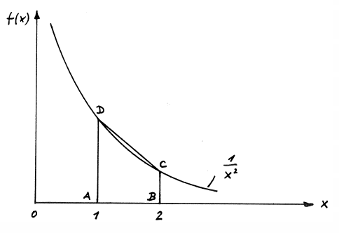
Figure 1.1: Principle of numerical integration.

The 'numerical' result is in this case $0.625$ , i.e. we have introduced an (absolute) methodological error:

$\begin{equation} \epsilon_{p} = 0.5 - 0.625 = -0.125. \end{equation}$

Other typical methodological errors arise for example from the truncation of an infinite series (truncation error), and so on.

Roundoff errors

Roundoff errors derive from the fact that in a computer only a limited number of bits is available to represent a real number (or, better, its mantissa).

A simple example:

    Calculation "by Hand":            Computer (7 sign. digits):

      123456.789                         0.1234568E+06
   +       9.876543                   +  0.9876543E+01
   ----------------                   ----------------
      123466.665543                      0.1234667E+06

Another example: If we perform the calculation in the code block below, we expect that the answer will be 50*0.1 = 5.

<script> value = 0.1; sum = 0; for (i=0; i<50; i++) { sum = sum + value; } document.write(sum); </script>

Because of roundoff errors, the result is 4.999999999999998. The reason for this is that the number 0.1, which is representable without problems in a decimal system, is represented an infinitely repeating pattern of bits in binary.

$\begin{equation} 0.1_{10} = 0.000110011001100\ldots_{2} \end{equation}$