Experimental Laboratory Exercises
|
|
Experimental Laboratory Exercises | |
|
|
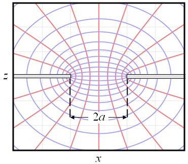
Maxwell contactConsider some material with a resistivity $\rho$ that is divided into two halves by an insulating membrane. If there is a circular hole of radius $a$ in the membrane then a current will flow through the hole when a voltage is applied across the membrane.
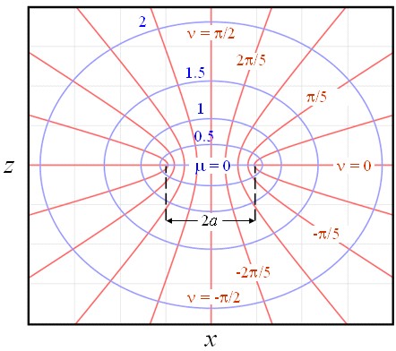
This problem was first considered in 1904 by Maxwell. [1] He showed that the resistance of the contact is $R=\rho/2a$. This is called the spreading resistance since it is associated with the current spreading out as it moves away from the hole. Most of the voltage drops where the current density is high near the hole. Far from the hole the current density approaches zero. The electric field is proportional to the current density so the electric field also approaches zero far from the hole. The electrostatic potential is the integral of the electric field. This approaches a constant far from the hole. To determine the potential $\phi$, Maxwell solved the Laplace equation for this geometry, $ \nabla^2\phi=0.$ It is convenient to solve this problem in oblate spheriodal coordinates $(\mu,\nu,\theta)$. These coordinates are defined as, $ x =a\text{cosh}\mu \cos \nu \cos\theta,$
In these coordinates, the potential is only a function of $\mu$. The Laplace equation in oblate spheriodal coordinates is, $\large \frac{1}{a^2 \left( \text{sinh}^2\mu+\sin^2\nu \right)}\left[\frac{1}{\text{cosh}\mu}\frac{\partial}{\partial\mu}\left(\text{cosh}\mu\frac{\partial\phi}{\partial\mu}\right)+\frac{1}{\cos\nu}\frac{\partial}{\partial\nu}\left(\cos\nu\frac{\partial\phi}{\partial\nu}\right)\right]+\frac{1}{a^2 \left( \text{cosh}^2\mu+\cos^2\nu \right)}\frac{\partial^2\phi}{\partial \theta^2}=0.$ Since $\phi$ is only a function of $\mu$, this reduces to, $\large \frac{\partial}{\partial\mu}\left(\text{cosh}\mu\frac{\partial\phi}{\partial\mu}\right)=0.$ This can be written as,
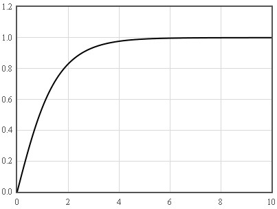
$\large \text{cosh}\mu\frac{d^2\phi}{d\mu^2}=-\text{sinh}\mu\frac{d\phi}{d\mu}.$ Let $y=\frac{d\phi}{d\mu}$. $\large \frac{dy}{d\mu}=-\text{tanh}\mu y.$ This equation can be solved by the separation of variables, $\large \frac{dy}{y}=-\text{tanh}\mu d\mu.$ Integrate, $ \ln y=-\ln\left(\text{cosh}\mu\right)+c_1.$ Here $c_1$ is an integration constant. Exponentiate the result, $ \large y=\frac{d\phi}{d\mu}=\frac{\exp(c_1)}{\text{cosh}\mu}.$ Integrate again, $ \phi=2\exp(c_1)\tan^{-1}\left(\text{tanh}\frac{\mu}{2}\right)+c_2.$ Here $c_2$ is another integration constant. It is always possible to add a constant to a potential so we can set $c_2=0$. The function $\tan^{-1}\left(\text{tanh}\frac{\mu}{2} \right)$ approaches $\pi/4$ for large $\mu$.
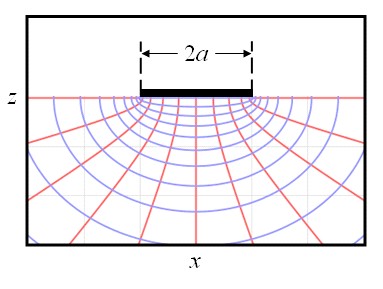
If some voltage $V/2$ is applied on one side of the membrane for very large $\mu$ and $-V/2$ is applied on the other side of the membrane for large $\mu$ then the potential that satisfies these boundary conditions is, $ \phi=\frac{2V}{\pi}\tan^{-1}\left(\text{tanh}\frac{\mu}{2}\right).$ It is straightforward to substitute this potential into the Laplace equation to verify that it is a solution. The electric field is the gradient of the potential. (The gradient in oblate spherical coordinates.) $ \large \vec{E}=-\nabla\phi=-\frac{V\text{sech}\mu}{\pi a\sqrt{\text{sinh}^2\mu+\sin^2\nu}}\hat{\mu}.$ The current density is simply proportional to the electric field, $ \large \vec{j}=-\frac{\vec{E}}{\rho}=\frac{V\text{sech}\mu}{\pi a \rho \sqrt{\text{sinh}^2\mu+\sin^2\nu}}\hat{\mu}.$ At $z=0$, $\mu=0$ and the current density is, $ \large \vec{j}(z=0)=-\frac{V}{\pi a \rho \sin\nu}\hat{z}.$ To calculate the current that is passing through the hole we can integrate the current density over the hole. At $z=0$, the current density only points in the $z$-direction. Furthermore, the current density does not depend on $\theta$; it is cylindrically symmetric around the $z$ axis. The current density only depends on the distance from the $z$-axis, $s=\sqrt{x^2+y^2}$. The current is, $ I=\int\limits_0^a 2\pi j(s)sds.$ Because of the cylindrial symmetry, the integration can be performed in the $x$-direction, $ \large I=-2\pi \int\limits_0^a \frac{V}{\pi a \rho \sin\nu}xdx.$ At $z=0$, $x=a\cos\nu$ and $dx=-a\sin\nu d\nu$. $\large I=2\pi \int\limits_{\pi/2}^0 \frac{Va\cos\nu}{\pi \rho } d\nu=\frac{2aV}{\rho}.$ The spreading resistance is the voltage divided by the current, $\large R=\frac{\rho}{2a}.$ It is convenient to use this result to rewrite the expressions for the potential, the electric field, and the current density in terms of the total current $I$. $ \phi=\frac{\rho I}{\pi a}\tan^{-1}\left(\text{tanh}\frac{\mu}{2}\right).$ $ \large \vec{E}=-\frac{\rho I \text{sech}\mu}{2\pi a^2 \sqrt{\text{sinh}^2\mu+\sin^2\nu}}\hat{\mu}.$ $ \large \vec{j}=\frac{I \text{sech}\mu}{2\pi a^2 \sqrt{\text{sinh}^2\mu+\sin^2\nu}}\hat{\mu}.$ Notice that the current density does not depend on the resistivity. This means that if there is a material with resistivity $\rho_1$ on one side of the membrane and a resistivity $\rho_2$ on the other side of the membrane that we can solve for the potentials on the two sides of the membrane independently. The spreading resistance in this case is, $\large R=\frac{\rho_1+\rho_2}{4a}.$ If there is a highly conductive material on one side of the membrane and a poorly conducting material on the other side, $\rho_1 << \rho_2$, then the spreading resistance is, $\large R=\frac{\rho_2}{4a}.$ This formula is used to determine the resistivities of semiconductors when a round metal contact is placed on the surface of a semiconductor.
In this calculation, we used Ohm's law $\rho\vec{j}=\vec{E}$. This means that the transport is assumed to be in the diffusive limit. For this to be true, $a$ should be larger than the electron mean free path $l$. If $a$ is on the order of $l$, then modifications of this result described by Sharvin [2] and Wexler [3] need to be considered. A further discussion of electrical contacts can be found in references [4-6].
[2] Yu. V. Sharvin, A possible method for studying Fermi surfaces, Sov. Phys. JETP 21 p. 655 (1965). [3] G Wexler, "The size effect and the non-local Boltzmann transport equation in orifice and disk geometry," Proc. Phys. Soc. 89 927 (1966). [4] R. Holm, Electrical Contacts, Springer, 2000. [5] P. G. Slade (editor), Electrical Contacts, Marcel Dekker, 1999. [6] M. Bruanovic, V.V. Konchits, N.K. Myshkin, Electrical Contacts, CRC Press, London (2007). |