The goal of this excercise is to investigate the current-voltage characteristsics of three different diodes. For the measurements, the KEITHLEY 2636A sourcemeter (SMU) was used to record the current-voltage characteristics. A python script was used to control the sourcemeter, sweep the voltages and save the obtained data into a csv file. In addition, the data as well as the python script were uploaded to eLab. A pseudo script on how to upload measurement data to eLab can be found here. A guide on how to get started with computer supported measurement techniques using python can be found here.
The current voltage characteristic follows an exponential behavior which can be described by the Shockley equation:
\begin{equation} I(V) = I_S \cdot (\exp{(\frac{e \cdot V}{n \cdot k_B \cdot T})}-1) \end{equation}
Here, $I$ is the diode current, $V$ the applied voltage, $I_S$ the reverse saturation current, $n$ the nonideality factor, $e$ the elementary charge, $k_B$ the boltzmann constant and $T$ the temperature.Using the SMU for measuring voltages and currents, it is necessary to select a range for the current. Choosing a small range results in a high precision at small currents, at the cost of precision at higher currents. For high ranges it is vice versa. As the current rises exponentially with the applied voltage, it is impossible to measure the whole current-voltage characteristic precisely with only one value for the current range. In order to still measure the current-voltage characteristic precisely, different values for the current range are selected and the measurement repeated for every selected range. This is again done using the python script which can be found below.
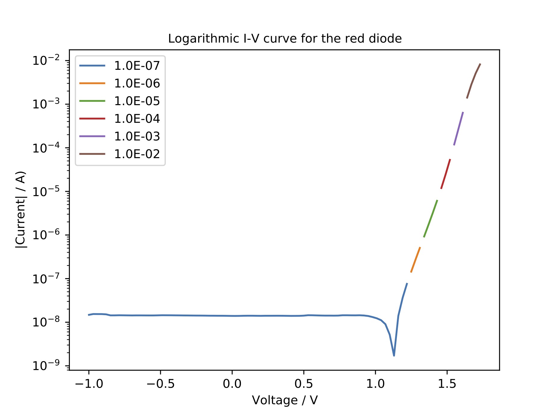
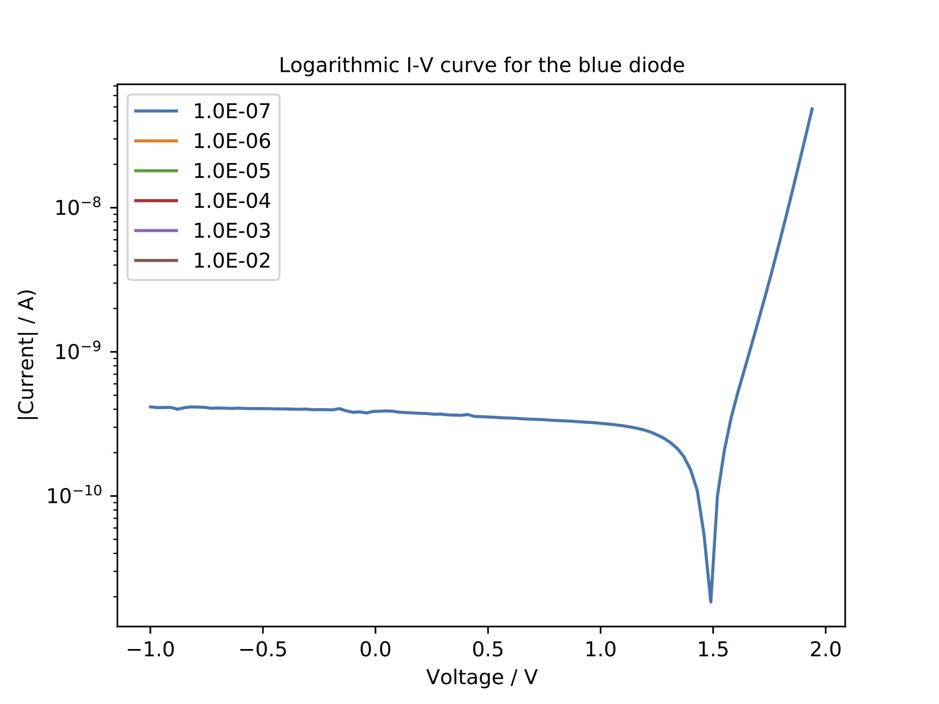
Plots of the obtained I-V curve as well as the raw data for the red and blue diodes are given below. As an exponential increase of the current with respect to the applied voltage is expected, the data is plotted on a semilogarithmic scale. Due to the negative current in the reverse bias regime, the absolute value of the current was taken. For better visualization, for each measurement only the parts of the current where the chosen range was suitable was plotted. The corresponding python file can be found below. Important to note is that at higher currents, the range did not really have an influence on the measurement whereas at lower currents, a smaller range did lead to a smaller offset from 0. The point where the current changes sign is visible as a kink in the plot. One would expect that this kink should be around 0 V. However, these kinks are at significantly higher voltages. For the red diode, they are found at around 1.1 V. For the blue diode, the kinks are between 1.4 to 1.8 V, depending on the range that was chosen. Due to this shift, only small currents were measured for the blue diode as the maximum applied voltage was kept fixed at two volts and the current started to rise just before this voltage. Therefore, only the measurement with the smallest current range lead to reliable results. For future experiments, it is suggested to adapt the voltage range to the shift of the IV-curve.
|
 |
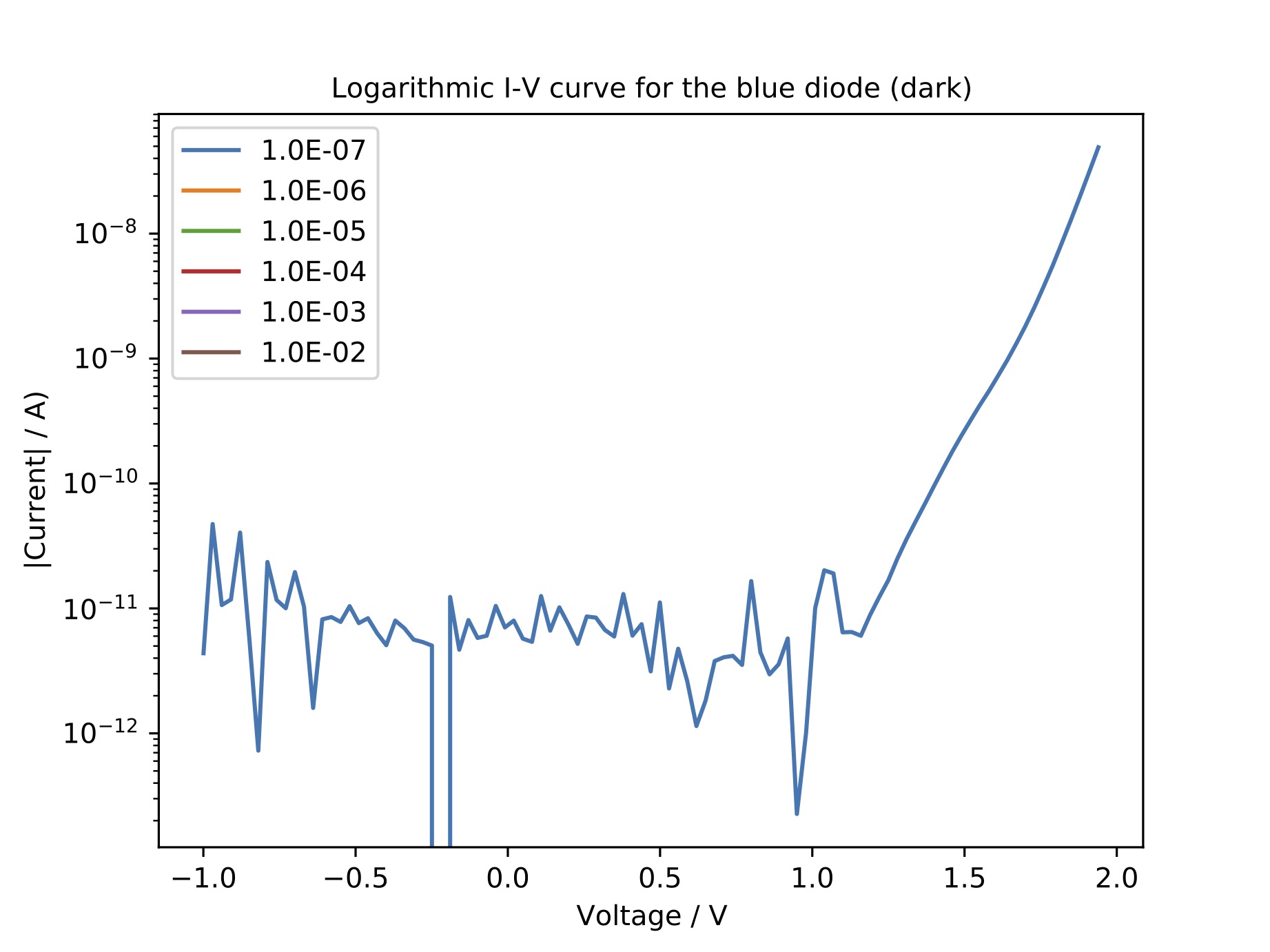
As the diode measurements were performed under daylight conditions, it was assumed that the photoelectric effect and the resulting phototcurrent are responsible for the shift of the zero point. Therefore, another measurement where the setup was placed into a spectacle case to block external light, was conducted. Again, a plot of the data as well as the raw data are found below. Looking at the I-V curves, one can see that the shift is still present. However, the current in reverse bias is significantly lower. Therefore, the measurement setup or the LED itself must be responsible for this effect. Examining the forward bias of the red diode in the logarithmic plot, one can see that the curve rises linearly in the beginning. This is the expected behaviour according to the Shockley equation. At higher voltages however, the curve starts to flatten out. This might be due to the non-ideality factor which in practice is a function of the applied voltage. As described elsewhere, the non-ideality factor increases with increasing voltage due to rising internal resistance. As a consquence, the slope of the logarithmic I-V curve decreases. A similar behavior is expected for the blue diode, however the choosen voltage range was to small for the observation of this effect.
 |
For the third diode, the UV-diode, an intersting behavior was observed. The current increased for positive as well as negative voltages. As the strong increase in current is already observed at relatively small negative voltages, it seems rather unlikely that this is an effect due to the breakdown of the diode. In addition, kinks that are related to a change of the sign of the current are found at positive as well as negative voltages (see raw data). This might indicate that the present UV diode does not consist of a single pn-junction but of different pn-junctions. These might be aligned in a way that regardless of how the voltage is applied, one of the junctions is forward biased similar to a two color LED as described here. To find out whether there are really two distinct LEDs or if the measured current was just the breakdown current one could conduct the following experiment. Light is only emitted if recombination occurs. In reverse bias, this is not the case. Therefore, one can apply positive and negative voltages at the diode and use some UV-fluorescent material to determine whether UV light is emitted in both cases or not. Despite the fact that the human eye cannot sense UV light, caution is required as the radiation can be harmful for the eyes. In addition, one can observe that the two arms of the curve do not have the same slope. For a better comparison, the data at higher currents is fitted to determine the saturation current and non-ideality factor.
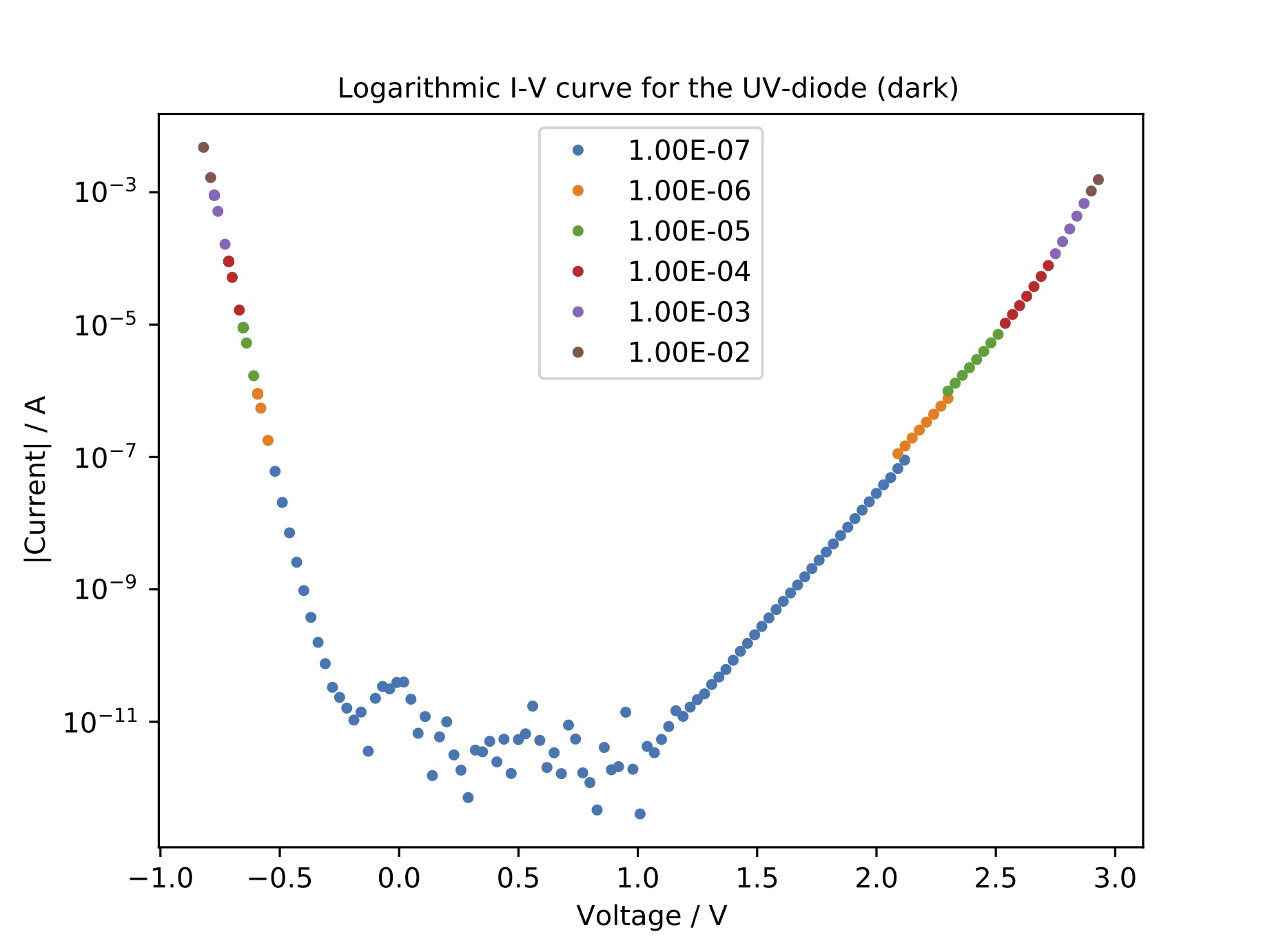 |
As already described above, the current-voltage characteristic of a diode can be described by the Shockley diode equation: \begin{equation} I(V) = I_S \cdot (\exp{(\frac{e \cdot V}{n \cdot k_B \cdot T})}-1) \end{equation} For higher currents, the -1 term can be neglected and after taking the logarithm on both sides, one obtains: \begin{equation} \ln{I} = \ln{I_S}+\frac{e \cdot V}{n\cdot k_B \cdot T} \end{equation} By plotting the curve in a semilogarithmic manner and fitting the linear relation above, one can determine the non-ideality factor $n$ and the saturation current $I_S$. The python script with the fit routine can be found below.
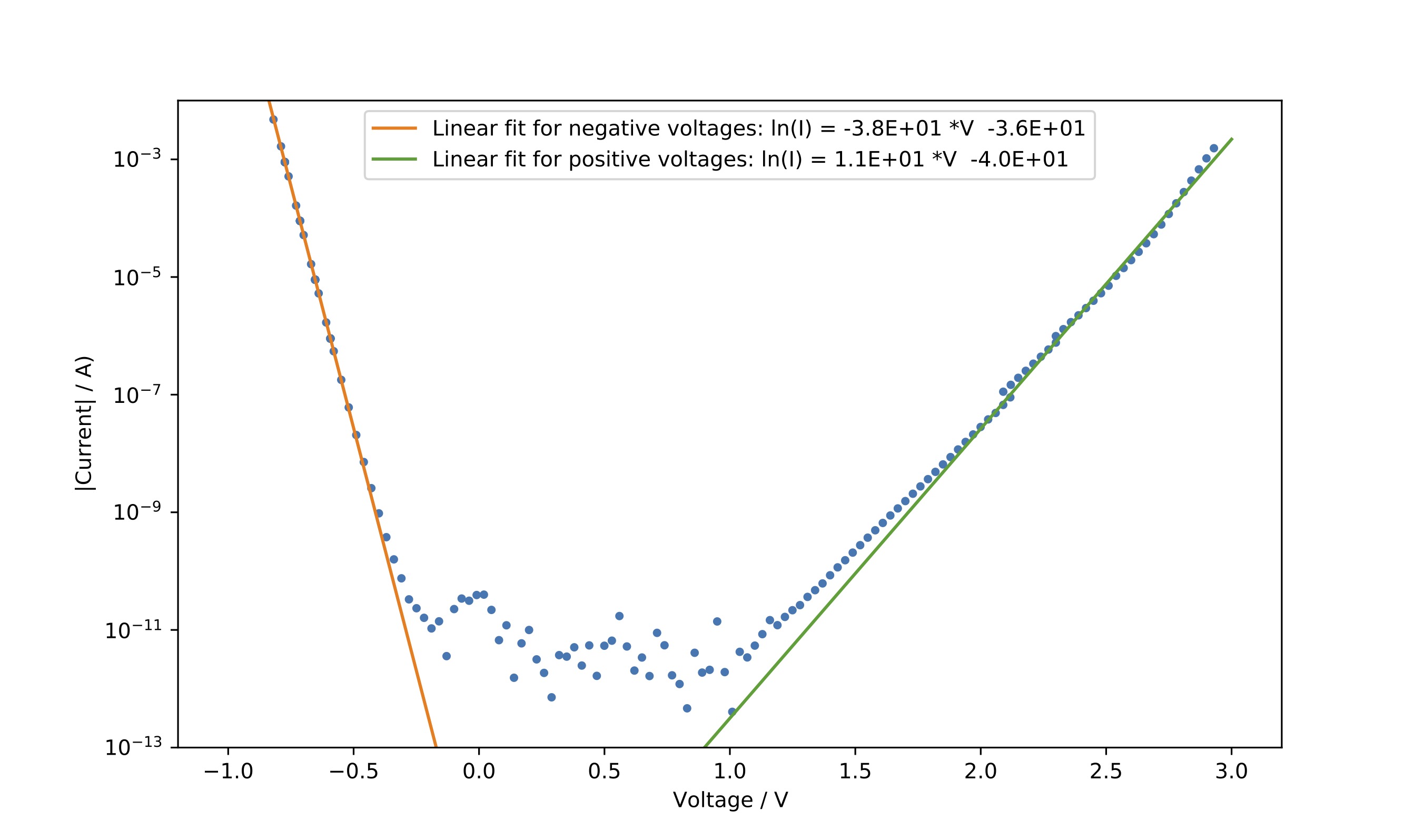
From the fit parameter, the saturation currents $I_S$ as well as the non-ideality factors are calculated. For the branch on the negative side one obtains: \begin{equation} I_S = 1.55 \cdot 10^{-16}~\mathrm{A}\\ n = 1.03 \end{equation} For the positive branch, one obtains: \begin{equation} I_S = 3.78 \cdot 10^{-18}~\mathrm{A}\\ n = 3.46 \end{equation} The calculated values for the saturation current seem rather small for light emitting diodes. The non-ideality factor however seems to be of the right magnitude as it usally varies between 1 and 2. Deviations might be the result of the measurement setup itself as well as the fact that the Shockley-equation is a simplified method to describe the highly complex transport of charge carriers inside a pn-junction.