PHY.K02UF Molecular and Solid State Physics

Fourier transforms

Consider a function $f\left(\vec{r}\right)$ that can be written in terms of plane waves,

$$ f\left(\vec{r}\right)= \int F\left(\vec{k}\right)e^{i\vec{k}\cdot\vec{r}}d\vec{k} .$$

This formula is known as the inverse Fourier transform in the [-1-1] notation (there is a discussion of Fourier transform notation below). The inverse transform constructs a real space function $f\left(\vec{r}\right)$ from a reciprocal space function $F\left(\vec{k}\right)$.

The Fourier transform that constructs a reciprocal space function is,

$$ F\left(\vec{k}\right)= \frac{1}{\left( 2\pi \right)^d} \int f\left(\vec{r}\right)e^{-i\vec{k}\cdot\vec{r}}d\vec{r},$$

where $d$ is the number of dimensions.

Example: a filter

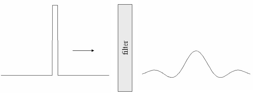
A square light pulse passes through a filter that only allows long wavelengths through. When the short wavelength components are removed by the filter, the pulse loses its sharp corners and the pulse broadens.

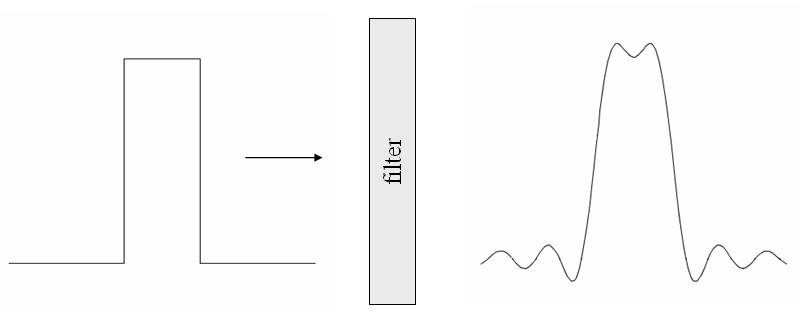
The pulse on the left has a of width $a$ and height 1 and can be described by the product of two Heaviside step functions, $f_L\left( x\right)=H\left( x/a + 0.5\right)H\left( 0.5-x/a\right)$. The Fourier transform of this pulse is,

\( F\left(k\right)= \frac{1}{2\pi} \int\limits_{-a/2}^{a/2} e^{-ikx}dx = \frac{\sin\left(ka/2\right)}{\pi k} \).

The orginal pulse can be recovered by taking the inverse Fourier transform.

\( f_L\left(x\right)= \int\limits_{-\infty}^{\infty} \frac{\sin\left(ka/2\right)}{\pi k} e^{ikx}dk \).

However, the filter prevents components with $|k| > k_0$ from passing through so the pulse on the right is,

\( f_R\left(x\right)= \int\limits_{-k_0}^{k_0} \frac{\sin\left(ka/2\right)}{\pi k} e^{ikx}dk = \frac{\text{Si}\left(k_0x+\frac{1}{2}\right) - \text{Si}\left(k_0x-\frac{1}{2}\right)}{\pi} \).

Here $\text{Si}\left(x\right)=\int\limits_0^x \frac{\sin x'}{x'}dx'$ is the sine integral.

Short pulses are made up of more short wavelength components. The filter removes more of a short pulse. When pulses are used for communication, they often travel as voltage pulses along a wire or as light pulses through an optical fiber. In both cases the pulses travel at about the speed of light. High data transmission rates are achieved by using short pulses. However, there more losses at high frequencies in a wire than in a optical fiber. The wire acts like a filter and it is not possible to transmit very short pulses. An optical fiber can transmit high frequency components and is called broadband. A broadband transmission channel can be used for high data rates.

In a diffraction experiment, the crystal acts like a filter for the waves passing through it. However, diffraction depends not just on the wavelength of the waves but also on the direction the waves are traveling. All of the information about the wavelength and the direction of the wave is contained in the wave vector $\vec{k}$.

Notation

There are several notations for Fourier transforms in use. The main differences in the notations are where factors of 2π are introduced. A general expression for the Fourier transform is, [MathWorld]

\( F_{a,b}\left(\vec{k}\right)=\mathcal{F}_{a,b}\{f\left(\vec{r}\right)\}= \sqrt{\frac{|b|^d}{\left( 2\pi \right)^{d\left(1-a\right)}}} \int\limits_{-\infty}^{\infty} f\left(\vec{r}\right)e^{ib\vec{k}\cdot\vec{r}}d\vec{r} \).

Here $a$ and $b$ are constants. $d$ is the number of dimensions that $\vec{r}$ is defined in. The corresponding inverse Fourier transform is,

\( f\left(\vec{r}\right) =\mathcal{F}^{-1}_{a,b}\{F\left(\vec{k}\right)\}=\sqrt{\frac{|b|^d}{\left( 2\pi \right)^{d\left(1+a\right)}}} \int\limits_{-\infty}^{\infty} F_{a,b}\left(\vec{k}\right)e^{-ib\vec{k}\cdot\vec{r}}d\vec{k} \).

In physics typically, $a=0$ and $b=-1$. In mathematics and systems engineering $a=1$ and $b=-1$ are used. In signal processing, $a=0$ and $b=-2\pi$ are used.

Notation [-1,-1]
Notation [-1,-1] was used above. It is the most logical when you think about a Fourier transform being the continuous sum of plane waves. In this notation, the Fourier transform of $f\left(\vec{r}\right)$ is,

\( F_{-1,-1}\left(\vec{k}\right)= \frac{1}{\left( 2\pi \right)^d} \int f\left(\vec{r}\right)e^{-i\vec{k}\cdot\vec{r}}d\vec{r} \).

The inverse Fourier transform is,

\( f\left(\vec{r}\right)= \int F_{-1,-1}\left(\vec{k}\right)e^{i\vec{k}\cdot\vec{r}}d\vec{k} \).

Notation [1,-1]
In notation [1,-1], the factor of $\left(2\pi\right)^d$ is moved from the formula for the Fourier transform to the formula for the inverse Fourier transform. This notation arises naturally in some diffraction problems. The Fourier transform of $f\left(\vec{r}\right)$ is,

\( F_{1,-1}\left(\vec{k}\right)= \int f\left(\vec{r}\right)e^{-i\vec{k}\cdot\vec{r}}d\vec{r} \).

The inverse Fourier transform is,

\( f\left(\vec{r}\right)= \frac{1}{\left( 2\pi \right)^d} \int F_{1,-1}\left(\vec{k}\right)e^{i\vec{k}\cdot\vec{r}}d\vec{k} \).

Matlab uses this notation.

Notation [0,-1]
In notation [0,-1], the factor of $\left(2\pi\right)^d$ is divided equally between the Fourier transform and inverse Fourier transform. The Fourier transform of $f\left(\vec{r}\right)$ is,

\( F_{0,-1}\left(\vec{k}\right)= \frac{1}{\left( 2\pi \right)^{d/2}} \int f\left(\vec{r}\right)e^{-i\vec{k}\cdot\vec{r}}d\vec{r} \).

The inverse transform is,

\( f\left(\vec{r}\right)= \frac{1}{\left( 2\pi \right)^{d/2}} \int F_{0,-1}\left(\vec{k}\right)e^{i\vec{k}\cdot\vec{r}}d\vec{k} \).

By default, Mathematica and Wolfram Alpha use [0,1] notation. It is like [0,-1] but the sign is opposite in the exponent.

Notation [0,-2π]
Notation [0,-2π] is popular in the engineering literature. In this notation, the Fourier transform of $f\left(\vec{r}\right)$ is,

\( F_{0,-2\pi}\left(\vec{q}\right)= \int f\left(\vec{r}\right)e^{-i2\pi\vec{q}\cdot\vec{r}}d\vec{r} \).

Here the wavelength is $\lambda= 1/|\vec{q}|$. The inverse transform is,

\( f\left(\vec{r}\right)= \int F_{0,-2\pi}\left(\vec{q}\right)e^{i2\pi\vec{q}\cdot\vec{r}}d\vec{q} \).

This notation is most often used in one-dimensional problems to calculate the Fourier transform of a function of space $f\left(x\right)$ or a function of time $f\left(t\right)$. For a one-dimensional function of space, the Fourier transform is,

\( F_{0,-2\pi}\left(q\right)= \int f\left(x\right)e^{-i2\pi qx}dx \).

The inverse transform is,

\( f\left(x\right)= \int F_{0,-2\pi}\left(q\right)e^{i2\pi qx}dq \).

For a function of time, $f\left(t\right)$ is expressed in terms of periodic functions $e^{i2\pi\nu t}$ where the relationship between the frequency $\nu$ and the period $T$ is, $\nu = 1/T$. The Fourier transform of $f\left(t\right)$ is,

\( F_{0,-2\pi}\left(\nu\right)= \int f\left(t\right)e^{-i2\pi \nu t}dt \).

The inverse transform is,

\( f\left(t\right)= \int F_{0,-2\pi}\left(\nu\right)e^{i2\pi \nu t}d\nu \).

Useful theorems

Linearity and superposition
$\mathcal{F}\{\alpha f\left(\vec{r}\right) +\beta g\left(\vec{r}\right)\} = \alpha\mathcal{F}\{f\left(\vec{r}\right)\} + \beta\mathcal{F}\{g\left(\vec{r}\right)\}$ where $\alpha$ and $\beta$ are any constants.

Similarity
$\mathcal{F}\{f\left(\frac{\vec{r}}{a}\right)\} = |a|^dF\left(a\vec{k}\right)$.

Shift
$\mathcal{F}\{f\left(\vec{r}-\vec{r}_0\right)\} = F\left(\vec{k}\right)\exp\left(-i\vec{k}\cdot\vec{r}_0\right)$.

Convolution

The convolution of functions $f(\vec{r})$ and $g(\vec{r})$ is defined as,

$$f*g = \int f(\vec{r}')g(\vec{r}-\vec{r}')d\vec{r}'.$$

In one dimension, $$f*g = \int\limits_{-\infty}^{\infty} f(x')g(x-x')dx'.$$

You can imagine sliding $g(x)$ past $f(x)$ and determining the area under the product at every point. The upper panel allows you to slide $g(x)$ past $f(x)$. The convolution is shown in the lower panel and the green line shows how far $g(x)$ is shifted with respect to $f(x)$.

$f(x')$
$g(x-x')$

$x'$

$x=$ 0

$f(x)*g(x)$

$x$

The convolution theorem states that the Fourier transform of the product of two functions is the convolution of their Fourier transforms (maybe with a factor of $2\pi$ or $\sqrt{2\pi}$ depending on which notation for Fourier transforms you use). There are similar convolution theorems for inverse Fourier transforms.

Notation [-1,-1]:  $\mathcal{F}\{fg\}=\mathcal{F}\{f\}*\mathcal{F}\{g\}$,  $\mathcal{F}^{-1}\{FG\}=\frac{1}{2\pi}\mathcal{F}^{-1}\{F\}*\mathcal{F}^{-1}\{G\}$.

Notation [1,-1]:  $\mathcal{F}\{fg\}=\frac{1}{2\pi}\mathcal{F}\{f\}*\mathcal{F}\{g\}$,  $\mathcal{F}^{-1}\{FG\}=\mathcal{F}^{-1}\{F\}*\mathcal{F}^{-1}\{G\}$.

Notation [0,-1]:  $\mathcal{F}\{fg\}=\frac{1}{\sqrt{2\pi}}\mathcal{F}\{f\}*\mathcal{F}\{g\}$,  $\mathcal{F}^{-1}\{FG\}=\frac{1}{\sqrt{2\pi}}\mathcal{F}^{-1}\{F\}*\mathcal{F}^{-1}\{G\}$.

Notation [0,-2π]:  $\mathcal{F}\{fg\}=\mathcal{F}\{f\}*\mathcal{F}\{g\}$,  $\mathcal{F}^{-1}\{FG\}=\mathcal{F}^{-1}\{F\}*\mathcal{F}^{-1}\{G\}$.

Table of Fourier transforms

The Fourier transforms of some functions in the four notations are given in the table below.

 $\large f\left(\vec{r}\right)$ 

 $\large F_{-1,-1}\left(\vec{k}\right)$ 

 $\large F_{1,-1}\left(\vec{k}\right)$ 

 $\large F_{0,-1}\left(\vec{k}\right)$ 

 $\large F_{0,-2\pi}\left(\vec{q}\right)$ 

 $\large \exp\left( - \left(\frac{x}{a}\right)^2\right)$ 

 $\large \frac{a}{2\sqrt{\pi}}\exp\left(-\frac{a^2k^2}{4}\right)$ 

 $\large a\sqrt{\pi}\exp\left(-\frac{a^2k^2}{4}\right)$ 

 $\large \frac{a}{\sqrt{2}}\exp\left(-\frac{a^2k^2}{4}\right)$ 

 $\large a\sqrt{\pi}\exp\left(-\pi^2a^2q^2\right)$ 

 $\large \exp\left(ik_0x\right)$ 

 $\large \delta\left(k-k_0\right)$ 

 $\large 2\pi\delta\left(k-k_0\right)$ 

 $\large \sqrt{2\pi}\delta\left(k-k_0\right)$ 

 $\large 2\pi\delta\left(2\pi q-k_0\right)$ 

 $\large \sin\left(k_0x\right)$ 

 $\large \frac{i}{2}\left(\delta\left(k+k_0\right)-\delta\left(k-k_0\right)\right)$ 

 $\large i\pi\left(\delta\left(k+k_0\right)-\delta\left(k-k_0\right)\right)$ 

 $\large i\sqrt{\frac{\pi}{2}}\left(\delta\left(k+k_0\right)-\delta\left(k-k_0\right)\right)$ 

 $\large i\pi\left(\delta\left(2\pi q+k_0\right)-\delta\left(2\pi q-k_0\right)\right)$ 

 $\large \cos\left(k_0x\right)$ 

 $\large \frac{1}{2}\left(\delta\left(k+k_0\right)+\delta\left(k-k_0\right)\right)$ 

 $\large \pi\left(\delta\left(k+k_0\right)+\delta\left(k-k_0\right)\right)$ 

 $\large \sqrt{\frac{\pi}{2}}\left(\delta\left(k+k_0\right)+\delta\left(k-k_0\right)\right)$ 

 $\large \pi\left(\delta\left(2\pi q+k_0\right)+\delta\left(2\pi q-k_0\right)\right)$ 

 $\large \exp\left(-|a|x\right)$  

 $\large \frac{|a|}{\pi\left(a^2+k^2\right)}$ 

 $\large \frac{2|a|}{a^2+k^2}$ 

 $\large \frac{\sqrt{2}|a|}{\sqrt{\pi}\left(a^2+k^2\right)}$ 

 $\large \frac{2|a|}{a^2+4\pi^2q^2}$ 

 $\large \text{sgn}\left(x\right)$  
$\text{sgn}\left(x\right)=-1$ for $x < 0$ and $\text{sgn}\left(x\right)=1$ for $x > 0$

 $\large \frac{-i}{\pi k}$ 

 $\large \frac{-2i}{k}$ 

 $\large \frac{-i\sqrt{2}}{\sqrt{\pi} k}$ 

 $\large \frac{-i}{\pi q}$ 

 $\large H(x)$ 

 $\large \frac{\delta (k)}{2}-\frac{i}{2\pi k}$ 

 $\large \pi \delta (k) -\frac{i}{k}$ 

 $\large \sqrt{\frac{\pi}{2}}\delta (k) -\frac{i}{\sqrt{2\pi} k}$ 

 $\large \frac{\delta(q)}{2}-\frac{i}{2\pi q}$ 

 $\large \text{sgn}\left(x\right)\exp\left(-|a|x\right)$  

 $\large \frac{-ik}{\pi\left(a^2+k^2\right)}$ 

 $\large \frac{-i2k}{a^2+k^2}$ 

 $\large \frac{-i\sqrt{2}k}{\sqrt{\pi}\left(a^2+k^2\right)}$ 

 $\large \frac{-i4\pi q}{a^2+4\pi^2q^2}$ 

 $\large H\left(x\right)\exp\left(-|a|x\right)$  

 $\large \frac{|a|-ik}{2\pi\left(a^2+k^2\right)}$ 

 $\large \frac{|a|-ik}{a^2+k^2}$ 

 $\large \frac{|a|-ik}{\sqrt{2\pi}\left(a^2+k^2\right)}$ 

 $\large \frac{|a|-i2\pi q}{a^2+4\pi^2q^2}$ 

 $\large \sqcap(x)=H\left(x+\frac{1}{2}\right)H\left(\frac{1}{2}-x\right)$ 
Square pulse: height = 1, width = 1, centered at $x=0$.

 $\large \frac{\sin\left(k/2\right)}{\pi k}$ 

 $\large \frac{2\sin\left(k/2\right)}{k}$ 

 $\large \frac{\sqrt{2}\sin\left(k/2\right)}{\sqrt{\pi} k}$ 

 $\large \frac{\sin\left(\pi q\right)}{\pi q}$ 

 $\large \sqcap \left(\frac{x-x_0}{a}\right)$ 
Square pulse: height = 1, width = $a$, centered at $x_0$.

 $\large \frac{\sin\left(ka/2\right)}{\pi k}\exp\left(-ikx_0\right)$ 

 $\large \frac{2\sin\left(ka/2\right)}{k}\exp\left(-ikx_0\right)$ 

 $\large \frac{\sqrt{2}\sin\left(ka/2\right)}{\sqrt{\pi} k}\exp\left(-ikx_0\right)$ 

 $\large \frac{\sin\left(\pi qa\right)}{\pi q}\exp\left(-i2\pi qx_0\right)$ 

 $\large \exp\left(i\vec{k}_0\cdot\vec{r}\right)$ 
Plane wave

 $\large \delta\left(\vec{k}-\vec{k}_0\right)$ 

 $\large \left(2\pi\right)^d\delta\left(\vec{k}-\vec{k}_0\right)$ 

 $\large \left(2\pi\right)^{d/2}\delta\left(\vec{k}-\vec{k}_0\right)$ 

 $\large \left(2\pi\right)^d\delta\left(2\pi\vec{q}-\vec{k}_0\right)$ 

 $\large 1$ 

 $\large \delta\left(k\right)$ 

 $\large 2\pi\delta\left(k\right)$ 

 $\large \sqrt{2\pi}\delta\left(k\right)$ 

 $\large \delta\left(q\right)$ 

 $\large \delta\left(x\right)$ 

 $\large \frac{1}{2\pi}$ 

 $\large 1$ 

 $\large \frac{1}{\sqrt{2\pi}}$ 

 $\large 1$ 

 $\large \delta\left(\frac{\vec{r}-\vec{r}_0}{a}\right)$ 

 $\large \left(\frac{a}{2\pi}\right)^d\exp\left(-i\vec{k}\cdot\vec{r}_0\right)$ 

 $\large a^d\exp\left(-i\vec{k}\cdot\vec{r}_0\right)$ 

 $\large \left(\frac{a}{\sqrt{2\pi}}\right)^d\exp\left(-i\vec{k}\cdot\vec{r}_0\right)$ 

 $\large a^d\exp\left(-i2\pi\vec{q}\cdot\vec{r}_0\right)$ 

 $\large \exp\left( - \frac{|\vec{r}-\vec{r}_0|^2}{a^2}\right)$ 

 $\large \left(\frac{a}{2\sqrt{\pi}}\right)^d\exp\left(-\frac{a^2k^2}{4}\right)\exp\left(-i\vec{k}\cdot\vec{r}_0\right)$ 

 $\large \left(a\sqrt{\pi}\right)^d\exp\left(-\frac{a^2k^2}{4}\right)\exp\left(-i\vec{k}\cdot\vec{r}_0\right)$ 

 $\large \left(\frac{a}{\sqrt{2}}\right)^d\exp\left(-\frac{a^2k^2}{4}\right)\exp\left(-i\vec{k}\cdot\vec{r}_0\right)$ 

 $\large \left( a\sqrt{\pi}\right)^d\exp\left(-\pi^2a^2q^2\right)\exp\left(-i2\pi \vec{q}\cdot\vec{r}_0\right)$ 

 $\large H(R-|\vec{r}-\vec{r}_0|)$ 
Disc of radius $R$ centered at $\vec{r}_0$, $\vec{r}\in \text{R}^2$

 $\large \frac{R}{2\pi |\vec{k}|} J_1 (|\vec{k}|R)\exp (-i\vec{k}\cdot\vec{r}_0)$ 

 $\large \frac{2\pi R}{|\vec{k}|} J_1 (|\vec{k}|R)\exp (-i\vec{k}\cdot\vec{r}_0)$ 

 $\large \frac{R}{|\vec{k}|} J_1 (|\vec{k}|R)\exp (-i\vec{k}\cdot\vec{r}_0)$ 

 $\large \frac{R}{|\vec{q}|} J_1 (2\pi |\vec{q}|R)\exp (-i2\pi \vec{q}\cdot\vec{r}_0)$ 

 $\large H(R-|\vec{r}-\vec{r}_0|)$ 
Sphere of radius $R$ centered at $\vec{r}_0$, $\vec{r}\in \text{R}^3$

 $\large \frac{1}{(2\pi )^3|\vec{k}|^3} \left(\sin (|\vec{k}|R) - |\vec{k}|R\cos (|\vec{k}|R)\right)\exp (-i\vec{k}\cdot\vec{r}_0)$ 

 $\large \frac{4\pi}{|\vec{k}|^3} \left(\sin (|\vec{k}|R) - |\vec{k}|R\cos (|\vec{k}|R)\right)\exp (-i\vec{k}\cdot\vec{r}_0)$ 

 $\large \frac{\sqrt{2}}{\sqrt{\pi}|\vec{k}|^3} \left(\sin (|\vec{k}|R) - |\vec{k}|R\cos (|\vec{k}|R)\right)\exp (-i\vec{k}\cdot\vec{r}_0)$ 

 $\large \frac{1}{2\pi^2 |\vec{q}|^3} \left(\sin (2\pi |\vec{q}|R) - 2\pi |\vec{q}|R\cos (2\pi |\vec{q}|R)\right)\exp (-i2\pi \vec{q}\cdot\vec{r}_0)$ 

Here $H\left(x\right)$ is the Heaviside step function, $\delta\left(x\right)$ is the Dirac delta function, $J_1(x)$ is the first order Bessel function of the first kind, and $d$ is the number of dimensions $\vec{r}$ is defined in. There is a longer table of functions like this at the bottom of the page, https://en.wikipedia.org/wiki/Fourier_transform.

Numerical Calculations of Fourier Transforms
Fourier analysis of real data sets, digital filtering
Discrete Fourier Transforms