A layered material can act like a filter for light. When light strikes the interface between two materials with different indices of refraction, part of the light is transmitted and part is reflected. In layered materials, there are reflections from each layer. Most of the time, the reflections from the different layers add incoherently, but under certain conditions the reflections add constructively. When this happens, the layered material acts like a mirror for a particular range of frequencies. It completely reflects certain frequencies while letting others pass through. This kind of structure is called a distributed Bragg reflector and is often used as part of surface emitting lasers.

Consider a simple layered material where the speed of light has different values in the different layers.

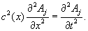
To determine the frequencies that would be reflected from this layered material, we start with the wave equation. For waves propagating in the x-direction the wave equation would be,

[1]

Here c(x) is the speed of light as a function of position, and A_j (j = y,z) are the components of the vector potential in the y and z directions.

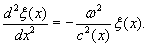
The wave equation is a partial differential equation that can be solved by the method of separation of variables. The normal mode solutions have the form A_j = ξ(x)e^-iωt. In a normal mode, all components oscillate with the same frequency ω. The quantity ξ satisfies the second order ordinary differential equation,

[2]

The subscript j is now suppressed since the equations for the two polarizations are the same. This is a second order ordinary differential equation with periodic coefficients known as Hill's equation. Sinusoidal waves only solve Eq. [2] if the speed of light is a constant everywhere. This means that for a layered material, the normal mode solutions won't have a clearly defined wavelength.

Because of the translational symmetry in this problem, the normal modes will be eigenfunctions of the translation operator T that shifts the solutions by one period, Tf(x) = f(x + a). Instead of trying to solve the wave equation directly, we will determine the eigenfunctions of the translation operator. This is a common practice in solid state physics. Notice that any function of the form,

[3]

is an eigenfunction of the translation operator with eigenvalue e^ika.

[4]

In solid state physics, functions like [3] are said to have Bloch form (after Felix Bloch who described electron wavefunctions in crystals). In mathematics, that the solutions to Hill's equation have this form is known as Floquet's theorem. The convention for describing waves in a periodic medium is to express them in terms of the eigenfunctions of the translation operator. These eigenfunctions have a well defined frequency and form a complete set that can be used to describe any wave. An eigenfunction is specified by the k that appears in the expression for the eigenvalue. It turns out that the physical interpretation of k is nearly the same as the wavenumber of harmonic waves (usually also called k).

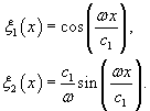
We proceed by constructing the translation operator. To do this we need two linearly independent solutions of Eq. [2]. A convenient choice is specified by the boundary conditions,

[5]

For 0 > x > b with these boundary conditions, the solutions are

[6]

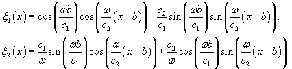
Using these expressions, the ξ functions and their derivatives at x = b can be determined. The values at x = b can then be used as the boundary conditions to specify the functions in the region b > x > a. The solutions are,

[7]

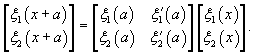
Now we have determined ξ₁(x) and ξ₂(x) in the region 0 > x > a. Any other solution can be written as a linear combination of these two solutions. In particular, ξ₁(x + a) and ξ₂(x + a) can be written in terms of ξ₁(x) and ξ₂(x). These two sets of solutions are related by the translation operator,

[8]

The elements of the translation matrix can be determined by evaluating Eq. [8] and its derivative at x = 0.

[9]

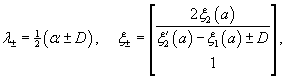
It is then straightforward to calculate the eigenvalues λ_± and eigenvectors of the translation operator. They are,

[10]

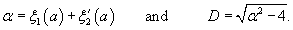
where

[11]

If |α| > 2, then the eigenvalues of the translation operator are real and one of them is greater than one while the other is less than one. This means that one of the eigenfunction solutions increases exponentially as a function of position while the other decays exponentially as a function of position. A solution that propagates through the crystal would have a constant amplitude so |α| > 2 corresponds to the situation where light is reflected out of the layered material. On the other hand if |α| < 2, the two eigenvalues are a complex conjugate pair on the unit circle. This means that every time the translation operator is applied the amplitude of the wave does not change; it just acquires a phase factor. By plotting α as a function of frequency, we can distinguish which frequencies will pass through the layered material (|α| < 2) and which will be reflected (|α| > 2).

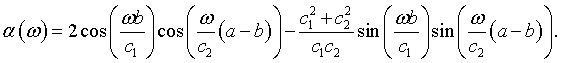
The relationship between α and frequency is,

[12]

This relationship is plotted in the Fig. 1.

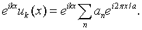
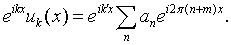
The eigenfunctions ξ₊ and ξ_- have Bloch form e^ikxu_k(x) where u_k(x) = u_k(x + a) is a periodic function. If |α| < 2, ξ₊ and ξ_- are complex and correspond to waves that can propagate through the material. In this case, the real part of the eigenfunctions is plotted in red and the imaginary part is plotted in blue. Since the vector potential cannot be imaginary, the real part and the imaginary part of the eigenfunctions are two independent solutions for the vector potential. If |α| > 2, the eigenfunctions ξ₊ and ξ_- are real and one decays exponentially while the other grows exponentially.

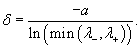
If we consider light striking an infinitely thick layered material, the only physically relevant solution for |α| > 2 is the exponentially decaying solution. The decay is described by e^-x/δ where δ is,

[13]

Figure 3 shows the decay length in units of the lattice constant a. Light is reflected for frequencies with a gray background and is transmitted for frequencies with a white background.

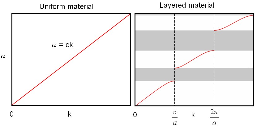
When light waves can propagate through the layered material (|α| < 2) they have the form, e^{i(kx - ωt)}u_k(x). The relationship between ω and k is called the dispersion relation. In a uniform material, the dispersion relation is a straight line with a slope corresponding to the speed of light in that medium, ω = ck. This is illustrated in the figure below on the left. The dispersion relation on the right is for a layered material. In this case, the wave solutions are divided into bands. Waves with frequencies in the gray bands are reflected out of the layered material so deep inside the materials there are no waves with frequencies in this range. This is called a photonic band gap.

The spatial part of the waves are a periodic function times an envelope function e^ikxu_k(x). The apparent k value of the envelope function always lies in the first Brilluoin zone. The decomposition of ξ₊ into the factors e^ikx and u_k(x) is shown in Fig. 4.

The reason that k can always be chosen to be in the first Brillouin zone can be understood by writting the periodic part as a Fourier series.

[14]

If k lies outside the first Brillouin zone, it is possible to separate it into a part inside the first Brillouin zone plus an integer m times a primitive reciprocal lattice vector, k = k' + 2πm/a. In terms of k', the spatial part of the wave can be written as,

[15]

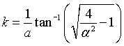
This is a periodic function with a period a times an envelope function with a wavenumber in the first Brillouin zone. Both descriptions (in terms of k and k') are equivalent. The formula for k as a function of wavenumber is,

[16]

The equivalence between the description in terms of k and k' is reflected in this formula. Because of the multivalued property of the inverse tangent, there are an infinite number of k's that solve this equation for a given ω. There is only one solution in the first Brillouin zone and the convention is to take that one.

The dispersion relation with k restricted to the first Brillouin zone is plotted below.

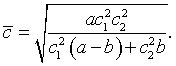
Near k = 0, the dispersion relation is nearly linear, ω = ck, and the waves travel with a speed c that is between the speeds of light in the two layers.

[17]

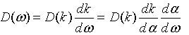
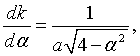
Since certain frequencies are forbidden, gaps appear in the density of states for this material. It is possible to calculate the density in states in terms of frequency, D(ω), from the density of states in k.

The possible k values are distributed uniformly in k. The density of states per unit length is,

[18]

The density of states in terms of frequency is,

[19]

where,

		[20]
	and	[21]

The density of states D(ω) is zero in the (gray) photonic band gaps and diverges at the edges of the band gaps where the slope of the dispersion relation dω/dk is zero.

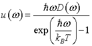
Once the density of states is known, it can be used to calculate any of the thermodynamic properties. The "tabulate D(ω)" button in Fig. 6 will generate a table of values for the density of states. This table can be input into collection of programs that calculate the thermodynamic properties of any system of noninteracting bosons from the density of states. The formulas for the thermodynamic properties and links to the programs are given below.

Energy spectral density:
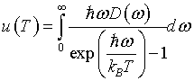
Internal energy density:
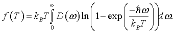
Helmholz free energy density:
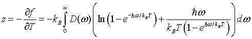
Entropy density:
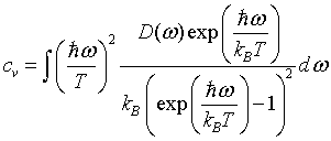
Specific heat: