Quantum mechanics can be used to calculate any property of a molecule. The energy $E$ of a wave function $\Psi$ evaluated for the Hamiltonian $H$ is,

\[ \begin{equation} E= \frac{\langle \Psi |H|\Psi\rangle}{\langle \Psi|\Psi\rangle}. \end{equation} \]

At first this seems like just a way to calculate the energy. However, this formula is used to calculate quantities like the bond length, the bond strength and the bond angles of a molecule. To calculate a bond length, the length is first guessed and the Hamiltonian for that bond length is constructed, the lowest energy wave function for this Hamiltonian is determined and the energy of this state is evaluated using the formula above. Then the Hamiltonian is adjusted to have little longer bond length or a little shorter bond length and the process is repeated until the bond length with the lowest energy is found. This is typically a computationally intensive process but it is remarkably accurate. Quantum mechanics is always correct. Discrepancies with experiment only appear when approximations are made to make the computation easier.

Many-particle Hamiltonian
The Hamiltonian that describes any molecule or solid is,

\[ \begin{equation} \label{eq:htotal} H_{\text{mp}}= -\sum\limits_i \frac{\hbar^2}{2m_e}\nabla^2_i -\sum\limits_a \frac{\hbar^2}{2m_a}\nabla^2_a -\sum\limits_{a,i} \frac{Z_ae^2}{4\pi\epsilon_0 |\vec{r}_i-\vec{r}_a|}+\sum\limits_{i< j} \frac{e^2}{4\pi\epsilon_0 |\vec{r}_i-\vec{r}_j|}+\sum\limits_{a< b} \frac{Z_aZ_be^2}{4\pi\epsilon_0 |\vec{r}_a-\vec{r}_b|} . \end{equation} \]

The first sum describes the kinetic energy of the electrons. The electrons are labeled with the subscript $i$. The second sum describes the kinetic energy of all of the atomic nuclei. The atoms are labeled with the subscript $a$. The third sum describes the attractive Coulomb interaction between the positively charged nuclei and the negatively charge electrons. $Z_a$ is the atomic number (the number of protons) of nucleus $a$. The fourth sum describes the repulsive electron-electron interactions. Notice the plus sign before the sum for repulsive interactions. The fifth sum describes the repulsive nuclei-nuclei interactions.

This Hamiltonian neglects some small details like the spin-orbit interaction and the hyperfine interaction. These effects will be ignored in this discussion. If they are relevant, they could be included as perturbations later. Remarkably, this Hamiltonian can tell us the shape of every molecule and the energy released (or absorbed) in a chemical reaction. Any observable quantity of any solid can also be calculated from this Hamiltonian. It turns out, however, that solving the Schrödinger equation associated with this Hamiltonian is usually terribly difficult. In brief, the Schrödinger equation is solved by guessing a wave function and then evaluating the energy with Eq. 1. Random guessing will not lead to a good solution quickly so routines that solve the Schrödinger equation employ some form of clever guessing. Here we will present an approach to determine approximate solutions to the Schrödinger equation by guessing that the many-electron solution can be written as a linear combination of suitably chosen atomic orbitals.

Born-Oppenheimer approximation
Since the nuclei are much heavier than the electrons, the electrons will move much faster than the nuclei. We may therefore fix the positions of the nuclei while solving for the electron states. The electron states are described by the electronic Hamiltonian $H_{\text{elec}}$.

\[ \begin{equation} \label{eq:helec} H_{\text{elec}}= -\sum\limits_i \frac{\hbar^2}{2m_e}\nabla^2_i -\sum\limits_{a,i} \frac{Z_ae^2}{4\pi\epsilon_0 |\vec{r}_i-\vec{r}_a|}+\sum\limits_{i< j} \frac{e^2}{4\pi\epsilon_0 |\vec{r}_i-\vec{r}_j|} +\sum\limits_{a< b} \frac{Z_aZ_be^2}{4\pi\epsilon_0 |\vec{r}_a-\vec{r}_b|}. \end{equation} \]

Reduced electronic Hamiltonian
The kinetic energy of the nuclei do not appear in $H_{\text{elec}}$ since the nuclei have been fixed. The last term in $H_{\text{elec}}$ does not depend on the positions of the electrons so it just adds a constant to the energy. Since a constant can always be added to or subtracted from the energy, this term will be neglected as we solve for the motion of the electrons. The electronic Hamiltonian cannot be solved analytically; it can only be solved numerically. To make further progress with an analytical solution, the electron-electron interaction term is neglected. This is not easily justified on physical grounds but this is the only known way to arrive at a reasonable analytic solution. When the electron-electron interactions are neglected, the reduced electronic Hamiltonian $H_{\text{elec}\_\text{red}}$ can be written as a sum of molecular orbital Hamiltonians $H_{\text{mo}}$.

\[ \begin{equation} \label{eq:helecred} H_{\text{elec}\_\text{red}}= -\sum\limits_i \frac{\hbar^2}{2m_e}\nabla^2_i -\sum\limits_{a,i} \frac{Z_ae^2}{4\pi\epsilon_0 |\vec{r}_i-\vec{r}_a|}= \sum\limits_i H_{\text{mo}}. \end{equation} \]

The eigenfunctions of this Hamiltonian can be found by the separation of variables. The many-electron wave functions are antisymmetrized products of the solutions to the molecular orbital Hamiltonian.

Molecular orbital Hamiltonian
The molecular orbital Hamiltonian describes the motion of a single electron in the potential created by all of the positive nuclei.

\[ \begin{equation} H_{\text{mo}}= - \frac{\hbar^2}{2m_e}\nabla^2 -\sum\limits_{a} \frac{Z_ae^2}{4\pi\epsilon_0 |\vec{r}-\vec{r}_a|}. \end{equation} \]

Note that while $H_{\text{elec}\_\text{red}}$ is a sum of molecular orbital Hamiltonians, all of these Hamiltonians are the same. Instead of having to solve a many-electron Hamiltonian, it is only necessary to solve a single one-electron Hamiltonian. This corresponds to a vast reduction in the computational effort required to solve the equations. The molecular orbitals play a similar role in describing the many-electron wave functions of molecules as the atomic orbitals do in describing the many-electron wave functions of atoms. There are various way to solve the molecular orbital Hamiltonian. Let's postpone the discussion of how to find the solutions of the molecular orbital Hamiltonian and just assume that we have found a set of eigenfunctions,

\[ \begin{equation} \label{eq:mo} H_{\text{mo}}\psi_n= E_n\psi_n . \end{equation} \]

A many-electron solution $\Psi$ that is constructed as an antisymmetrized product of molecular orbitals is an exact solution to $H_{\text{elec}\_\text{red}}$ and it is a good approximate solution to $H_{\text{elec}}$. It can be used to find the approximate energy of the many electron system using the equation,

\[ \begin{equation} E= \frac{\langle \Psi |H_{\text{elec}}|\Psi\rangle}{\langle \Psi|\Psi\rangle}. \end{equation} \]

As stated above, the shape of a molecule in terms of bond lengths and bond angles is determined by finding the arrangement of the atoms that minimizes this energy.

Bond potential
To calculate the bond potential, fix the nuclei of the two atoms involved in the bond at a certain distance apart and calculate the energy of the electronic Hamiltonian evaluated with the ground state many-electron wave function. Change the distance and recalculate the energy of the ground state. Repeat until the energy has been determined as a function of distance.

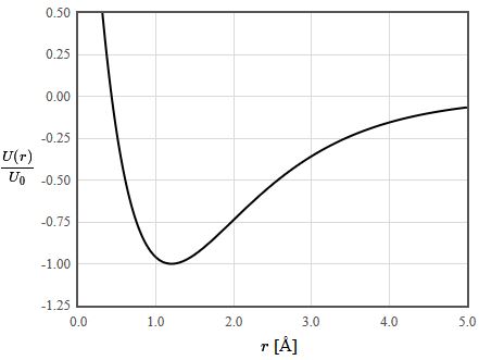
Bond length
The minimum of the bond potential gives the equilibrium bond length. Some books give tables of bond lengths for which provide an approximate value of the bond length. The bond length for a particular pair of atoms, like a carbon-carbon bond, is not always the same. It depends on the other atoms in the molecule.

Bond angle
Fix the nuclei at different bond angles and calculate the energy for each case. The bond angle with the lowest energy will be observed.

Shape of a molecule
The Schrödingrer equation can tell us if a molecule is linear or forms a ring. It can tell us the shape of a complicated molecule like a protein or DNA. To find the shape of a molecule, start with a guess for the shape and calculate the energy then make a small change in the shape and see if the energy decreases. The observed shape of the molecule will be at the energy minimum. There may be multiple energy minima resulting in different isomers of a molecule.

Rotational energy levels
The rotational levels of a diatomic molecule can be estimated by assuming that the atoms remain at their equilibrium spacing $r_0$ during rotation. In this can, the quantized energy levels of a rigid rotator can be used,

\[ \begin{equation} E_J= \frac{\hbar^2}{2I}J(J+1)= BJ(J+1), \end{equation} \]

where $I$ is the moment of inertia and $J$ is orbital quantum number, $J=0,1,2,\cdots$, and $B$ is called the rotational constant. For a diatomic molecule with an equilibrium spacing of the atoms of $r_0$ and atomic masses $m_a$ and $m_b$, the moment of inertia is $I=\frac{m_am_b}{m_a+m_b}r_0^2$.

The wave functions for a rigid rotor are the the spherical harmonics $Y_{Jm}(\theta,\phi)$. Here, $m$ is the quantum number characterizes the $z$-component of the molecule's angular momentum and takes on the values $m=-J,...,J$. Each rotational energy level has a degeneracy of $(2J+1)$.

Since photons have a spin of $1$, $J$ can only change by $\pm 1$ when photons are emitted or absorbed by a molecule.

A molecule with $N$ atoms has $3N$ degrees of freedom. There are always three are translational degrees of freedom which describe the motion of the center of mass of the molecule. A linear molecule (all of a the atoms are in a straight line) has two rotational degrees of freedom. If the atoms lie along the $x$-axis, there can be two different rotation speeds around the $y$- and $z$-axes. The atoms of a non-linear molecule do not all lie along a line and there are three rotational degrees of freedom.

Vibrational energy levels
For diatomic molecules, the bond potentials can be used to find the vibrational and rotational spectra of a molecule. Diatomic molecules only have one stretching mode where the two atoms in a molecule vibrate with respect to each other. In the simplest approximation, we imagine that the atoms are attached to each other by a linear spring. The spring constant can be determined from the bond potential. Near the minimum of the bond potential at $r_0$, the potential can be approximated by a parabola. This is the same potential as for a harmonic oscillator where the effective spring constant is $k_{\text{eff}}=\frac{d^2U}{dr^2}|_{r=r_0}$ and the reduced mass is $m_r=(1/m_a+1/m_b)^{-1}$. Here $m_a$ and $m_b$ are the masses of the two atoms. The angular frequency of this vibration is $\omega=\sqrt{k_{\text{eff}}/m_r}$. The vibrational modes of the molecule have the same energy level spectrum as a harmonic oscillator,

\[ \begin{equation} E_{\nu}=\hbar\omega(\nu+1/2) \hspace{1.5cm} \nu=0,1,2,\cdots. \end{equation} \]

The number of vibrational normal modes for a molecule with $N$ atoms is $3N-5$ for a linear molecule and $3N-6$ for a non-linear molecule.

Energy of a chemical reaction
Chemical reactions can be either exothermic (energy is released during the reaction) or endothermic (energy is absorbed during the reaction). To calculate how much energy is released or absorbed during a reaction, calculate the energies for all reactants and products. The change in energy during the reaction is the sum of the energies of the products minus the sum of energies of the reactants.

Speed of a chemical reaction
To calculate how long a chemical reaction takes, numerically integrate the time dependent Schrödinger equation for $H_{\text{total}}$ starting with the reactants nearby each other. This is an exceedingly computationally intensive calculation.

Molecular spectroscopy
Molecules can absorb a photon and make a transition between energy levels or they can emit a photon and make a transition between energy levels. Measuring the photon energies that are absorbed and emitted by molecules is an important way to study molecules experimentally. Transitions between rotational states occur by the absorption of microwave photons. Transitions between vibrational states occur by the absorption of infrared photons. Transitions between electronic states occur by the absorption of visible (or near visible) photons. The strength of an absorption or emission line depends on the rate for that transition. Transition rates are typically calculated using Fermi's golden rule,

$$\Gamma_{i\rightarrow f}= \frac{2\pi}{\hbar}\left|\langle f\left| H_1 \right|i\rangle\right|^2\delta (E_f-E_i).$$

The states $| i\rangle$ is the initial molecule + photon quantum state and $| f\rangle$ is the final molecular + photon quantum state and $H_1$ is the perturbation Hamiltonian. This perturbation Hamiltonian couples the molecular states of an isolated molecule to the photon field. Often the matrix element can be shown to be zero by symmetry. When this happens we say that the transition is forbidden. For more details see: Haken H., Christoph Wolf H. (1995) The Interaction of Molecules with Light: Quantum-Mechanical Treatment. In: Molecular Physics and Elements of Quantum Chemistry. Advanced Texts in Physics. Springer, Berlin, Heidelberg.

More accurate calculations
Ignoring the electron-electron interactions is a fairly crude approximation. There are more sophisticated methods like Hartree-Fock or density functional theory. These methods are not exact but do include the electron-electron interactions in an approximate form. There are many commercial and public domain programs available for these types of calculations.

Next: Calculate the molecular orbitals

---

• Demtröder, Kapitel 9 Atome, Moleküle und Festkörper
• A description of a quantum treatment of molecules can be found in Molecular Physics & Elementary of Quantum Chemistry by H. Haken and H. C. Wolf (The German version, Molekülphysik und Quantenchemie, is available as an ebook from the TU Graz library).
• A.Szabo and N. S. Ostlund, Modern Quantum Chemistry, McGraw-Hill, 1989.