If the amplitude of the periodic potential that an electron experiences is small, the solutions to the Schrödinger equation will be nearly the same as those for free electrons, and the dispersion relation will be nearly the parabolic free electron dispersion relation,

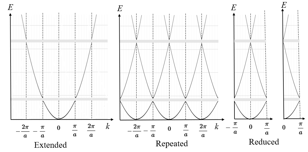
$$E=\frac{\hbar^2k^2}{2m}.$$

The dispersion curve will deviate from the free electron result near the Brillouin zone boundaries where $k$ satisfies the diffraction condition. At the Brillouin zone boundary, the group velocity $v_k = \frac{1}{\hbar}\frac{dE}{dk}$ goes to zero and the dispersion curve strikes the Brillouin zone boundary at 90°. This situation is illustrated as the extended zone scheme in the figure below. Small band gaps (shown in gray) appear in the dispersion relation.

The wave functions for any $k$ state will have Bloch form, $\psi = e^{ikx}u_k(x)$, where $u_k(x)$ is a periodic function. A periodic function can be expressed as a Fourier series, so the wave function can be written as,

$$\psi(x) = e^{ikx}\sum\limits_GC_Ge^{iGx}.$$

If we refer to the extended zone scheme and consider a $k$ in the second Brillouin zone $\left(\frac{\pi}{a} < k < \frac{2\pi}{a}\right)$, we could multiply $\psi(x)$ by $1 = e^{-i2\pi x/a}e^{i2\pi x/a}$. Since we multiply by one, the wave function $\psi$ does not change.

$$\psi(x) = e^{ikx}e^{-i2\pi x/a}e^{i2\pi x/a}\sum\limits_GC_Ge^{iGx}= e^{i(k-2\pi /a)x}\sum\limits_GC_Ge^{i(G+2\pi/a)x}.$$

The final form on the right has Bloch form, $\psi = e^{ik'x}u_{k'}(x)$, where $k' = k-2\pi /a$ is in the First Brillouin zone and $u_{k'}(x)$ must be a periodic function since it is expressed as a Fourier series. It is a different periodic function from $u_{k}(x)$. This means that we can assign any Bloch wave at any energy to a $k$ in the first Brillouin zone. If $k$ is initially outside the first Brillouin zone, it can be shifted by a reciprocal lattice vector back into the first Brillouin zone. The resulting $E\text{ vs. }k$ dispersion curve can be plotted by drawing a free-electron parabola at every reciprocal lattice point as shown in the repeated zone scheme. The repeated zone scheme is periodic, so all the information it contains is in the first Brillouin zone. This is the reduced zone scheme. For every $k$ state in the first Brillouin zone, there is a state with the same energy at $-k$ so it is only necessary to plot the reduced zone scheme for positive $k$.

Even though the extended zone scheme and the reduced zone scheme are equally valid, the reduced zone scheme is preferred because of how it simplifies the analysis of electronic transitions. If a visible or UV photon excites an electron from an initial (occupied) state into a final (empty) state, momentum must be conserved,

$$\hbar \vec{k}_{\text{photon}} + \hbar \vec{k}_{\text{initial}} = \hbar \vec{k}_{\text{final}} + \hbar \vec{G}.$$

The momentum of a visible photon is very small compared to the momentum of an electron, so it can be ignored and the conservation of momentum can be written,

$$\vec{k}_{\text{initial}} = \vec{k}_{\text{final}} + \vec{G}.$$

If two $k$-vectors that differ by a reciprocal lattice vector are plotted in the reduced zone scheme, they will have the same $k$ value in the first Brillouin zone. The electron will make a vertical transition from a lower band to a band at higher energy when it absorbs a photon.

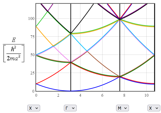
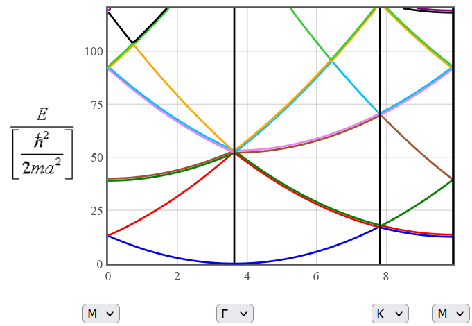
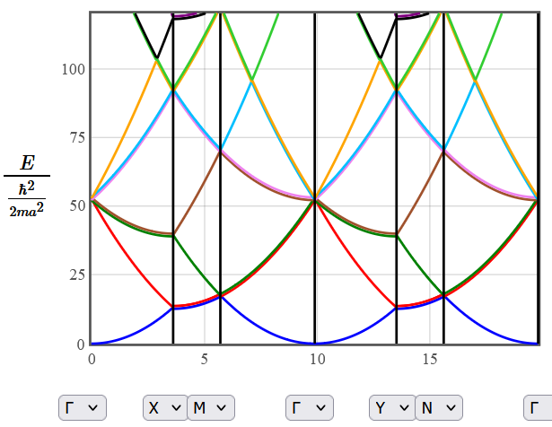
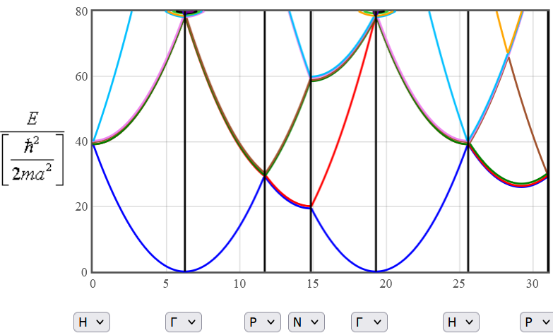
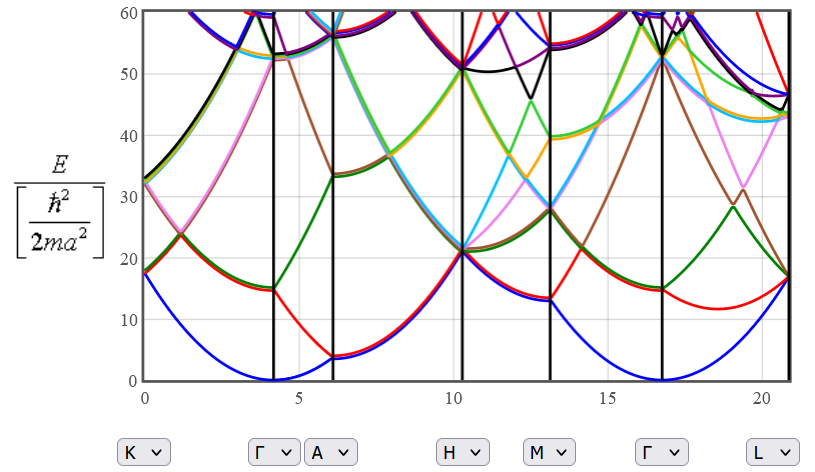
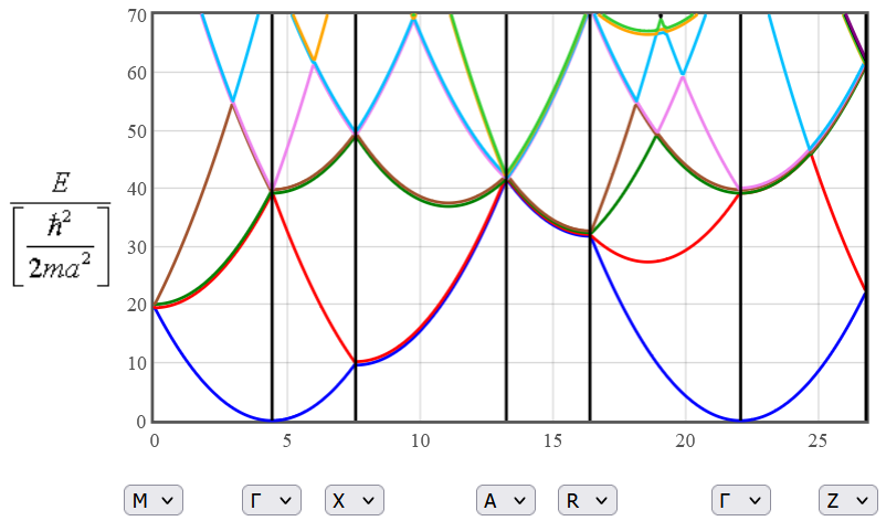
In two or three dimensions, the free-electron $E\text{ vs. }k$ dispersion curve is a paraboloid that can be centered at every reciprocal lattice vector to produce the repeated zone scheme. The formulas for these paraboloids are,

$$E =\frac{\hbar^2(\vec{k}+\vec{G})^2}{2m}.$$

There is one paraboloid for every reciprocal lattice vector. Cuts are made through this family of parabolas in the high symmetry directions of the first Brillouin zone to plot the dispersion relation in those directions.

1-D	2-D square
2-D hexagonal	General 2D lattice
Simple cubic	Face centered cubic
Body centered cubic	Hexagonal
Tetragonal	Body Centered Tetragonal
Orthorhombic	Simple Monoclinic

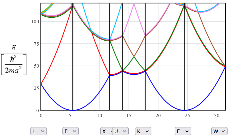
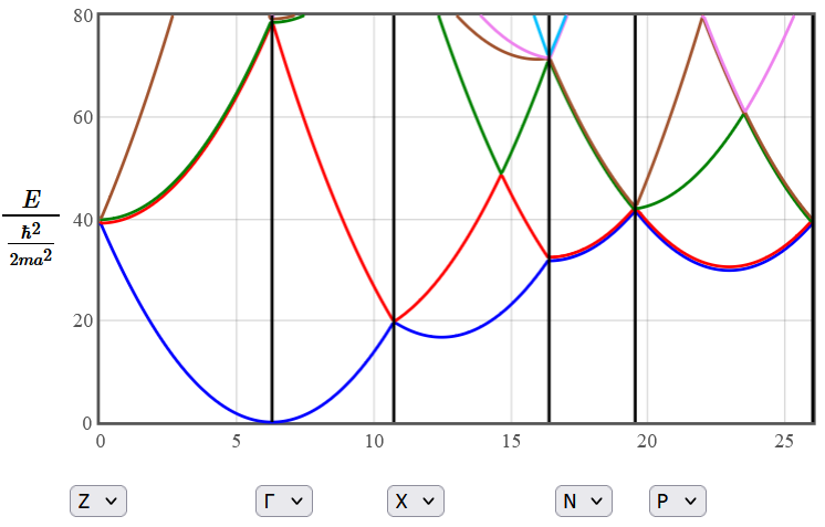
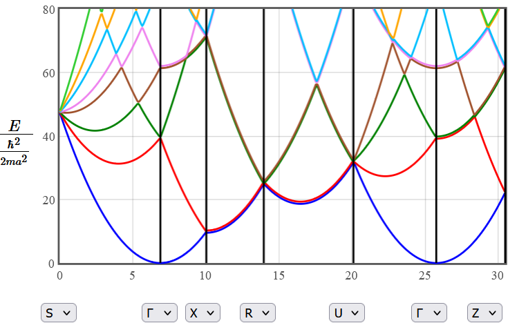
Some examples of the utility of the empty lattice approximation are shown below.

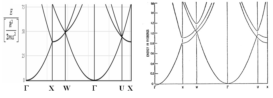
On the left is the empty lattice approximation for an fcc crystal and on the right is the calculated band structure of aluminum (an fcc metal). The right image was taken from W.A. Harrison, Physical Review, vol. 118 pp. 1182-1189 (1960).